
This page reviews the theory for the Bayer structure and provides comprehensive results for the Kodak image dataset. It also adapts results and terminology (LSLCD) from the recent paper "Least-Squares Luma-Chroma Demultiplexing Algorithm for Bayer Demosaicking" to appear in IEEE Transactions on Image Processing.
Geometric structure of the Bayer color-filter array
Formation and representation of the Bayer CFA image
Least-squares filter design for CFA signal demultiplexing
Least-squares luma-chroma demultiplexing (LSLCD) algorithm results
LSLCD optimization - quality vs complexity
The Bayer array pattern is regular and periodic and its geometric structure is the following:
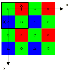
The Bayer sampling structure lies on an integer lattice Λ. The horizontal and vertical sampling spaces in this sampling structure are equal, the distance between them being X. X will be used as unit of length (pixel height, px).
The Bayer structure has three classes corresponding to the red (R), green (G) and blue (B) filters. The origin of the set is at the upper left corner with a green sample having a red sample to the right and a blue sample below. One period of the Bayer pattern determined by the sublattice Γ is indicated by the heavy square contour in the upper left corner.
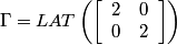
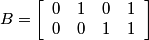
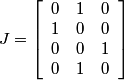
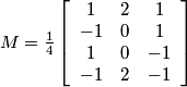
Following the chapter's theory and looking at the Bayer pattern above, one can come up with the following set of matrices:
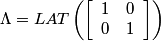 ,
,
 .
.
 .
.
 .
.
Column 2 of the J matrix represents the green in the Bayer structure.
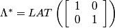
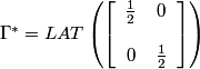
In the frequency domain, we have:
 ,
,
 .
.
 .
.
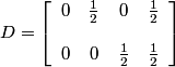
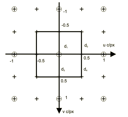
The reciprocal lattices Λ* (⊙) and Γ* (+) and a suitable choice of representatives for the cosets of Λ* in Γ* are illustrated below:
This gives:
 .
.
The four transformed signals qi are explicitly given by:
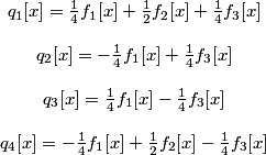 .
.
Noting that q3 = -q2 the pseudo inverse matrix is given by:
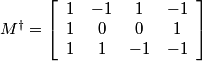 .
.
This gives an inverse relationship that, considering the constraint q3 = -q2, simplifies to :
 .
.
In the frequency domain, the four transformed signals are modulated at the frequencies (0.0, 0.0), (0.5, 0.0), (0.0, 0.5) and (0.5, 0.5) so that:
 .
.
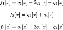
The Bayer power density spectrum of an image will look similar to the one below. The frequency components q1, q2 and q4 correspond respectively to the fL, fC2 and fC1 components. Note that there are two separate independent copies of Q2(u, v) at (0.5, 0.0) and (0.0, 0.5) respectively. On the figure these two different copies are marked as Q2 and Q3.
What is important to notice in this plot is that high frequency luma components overlap with high frequency chroma components. High frequency luma patterns intrude into the chrominance bands, resulting in false colors. High-frequency chrominance information intrudes into the luma band, resulting in false luma patterns, often having a zipper-like appearance.

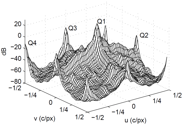
The first image shows the demosaicking result when only the C2a component (Q3) is used. The second image shows the demosaicking results when we use the C2b component (Q2) of the spectrum exclusively.
The idea behind demosaicking algorithms based on the frequency-domain representation is to extract the luma and modulated chrominance components from the CFA signal using spatial filters and then to transform the demodulated chrominance components to the desired tristimulus values. In the process, the specific structure of the CFA signal should be exploited.
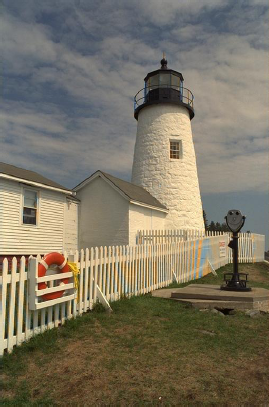
In the case of the Bayer sampling structure, one of the chroma components is modulated at two different frequencies: (0.5, 0.0) and (0.0, 0.5). Either one of these frequencies could be used to reconstruct the signal. However, if locally one suffers from crosstalk, the other one is relatively free of crosstalk. By adaptively selecting which of the two to use at each point, superior results are obtained.
The figures above illustrate schematically the local spectrum scenarios for the Bayer CFA. For the first scenario, Q2 is the better estimate. For the second one, we would rather use Q3.
Adaptive demosaicking algotithm for the Bayer CFA
1. Filter fCFA with a bandpass filter h4 centered at frequency (0.5, 0.5) to extract .
.
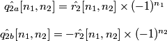 .
.
3. The local average energies eX and eY are estimated using modulated Gaussian filters with standard deviations of rG1 and rG2 px along major and minor axes, centered at frequencies (±um, 0.0) and (0.0, ±vm) c/px respectively. The filter at (0.0, ±vm) is the transpose of the filter at (±um, 0.0). This is followed by smoothing of the squared output with a 5 by 5 moving average filter.
4. Using the coefficinet w = eY / (eX + eY), the estimate of q2 is obtained as:
 .
.
5. The luma component is estimated by:
 .
.
6. Estimate RGB components ![]() from
from ![]() and
and ![]() .
.
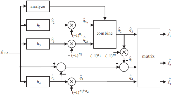
The block diagram of adaptive demosaicking algorithm for the Bayer CFA structure is below:
The filter design method is a crucial step for successful implementation of demosaicking algorithms. The method used to design these filters: Least Squares Luma Chroma Demultiplexing (LSLCD) has been explained in the book chapter (but not under that name). Assuming that the difference between the original image and its demultiplexed variant can be modeled as a stationary random field, the filters are designed such that they minimize the expected square error:

In practice, the original image is not available. The estimation error is minimised using a training set. In our experiments, the training set was one of the following:
For the Bayer pattern, the approach needs to be used to determine the three filters h2, h3 and h4. Beause h2 and h3 are both representatives of the chroma 2 component the least squares algorithm needs to be done simultaneously on both in order to minimize the squared error estimation of q2 (the procedure used to take both chroma components in consideration is explained above). The estimate of q2[n1, n2] then becomes:
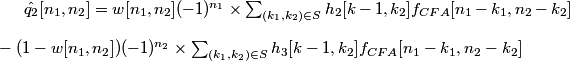 .
.
h2 and h3 can be chosen jointly to minimize the total
squared error between q2 and ![]() over the training
set. We cast this squared error in matrix form. Let h23 be the
2NB x 1 column vector obtained by stacking h2 on top of
h3. The column vector q(i)2 is obtained by
scanning the elements of q2[n1, n2] over W
(i). Finally, we form a NW x 2NB matrix
W(i) as follows: the first NB columns are formed by
reshaping w(i)[n1,
n2](-1)n1 f
(i)CFA[n1-k1,
n2-k2] for each (k1, k2) ∈S
while the second NB columns are formed by reshaping
-(1-w(i)[n1, n2])(-1)n2
f (i)CFA[n1-k1,
n2-k2] in the same order. This leads to a least squares
problem of the form:
over the training
set. We cast this squared error in matrix form. Let h23 be the
2NB x 1 column vector obtained by stacking h2 on top of
h3. The column vector q(i)2 is obtained by
scanning the elements of q2[n1, n2] over W
(i). Finally, we form a NW x 2NB matrix
W(i) as follows: the first NB columns are formed by
reshaping w(i)[n1,
n2](-1)n1 f
(i)CFA[n1-k1,
n2-k2] for each (k1, k2) ∈S
while the second NB columns are formed by reshaping
-(1-w(i)[n1, n2])(-1)n2
f (i)CFA[n1-k1,
n2-k2] in the same order. This leads to a least squares
problem of the form:
 .
.
Finally, h2 and h3 are extracted from h23 and reshaped to give the optimised filters h2[x] and h3[x].
An example the frequency response of the filters obtained using this procedure can be found here.
The recommended values for the various parameters and regions of support are:
A full list of results for the 24 Kodak images can be found here.
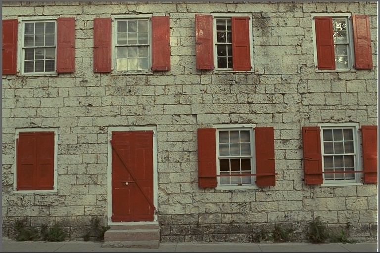
The table below shows the LSLCD algorithm results for the first 3 Kodak images. The training sets are chosen as follows:
| No. | Thumb | Original | A | B | C | D |
| 1 |  |
TIFF | TIFF
39.55 1.052 |
TIFF
38.67 1.133 |
TIFF
38.17 1.193 |
TIFF
37.92 1.190 |
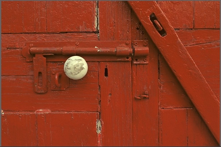
| 2 |  |
TIFF | TIFF
41.54 0.581 |
TIFF
40.81 0.642 |
TIFF
40.84 0.628 |
TIFF
40.65 0.664 |
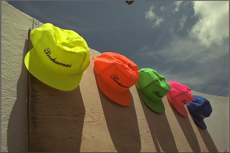
| 3 |  |
TIFF | TIFF
43.22 0.481 |
TIFF
43.37 0.509 |
TIFF
42.76 0.490 |
TIFF
42.22 0.512 |
The details of the complexity analysis can be found here. The quality versus complexity plots are presented below.
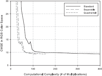
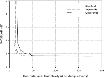
Following the analysis, we identify the configuration [ 5 5 9 3 11 1 ] as a good choice. This corresponds to a 5 x 5 least-squares filter h4, 9 x 3 least-squares filter h2, 3 x 9 least-squares filter h3, 11 x 1 Gaussian filter hG1 centered at (0.375, 0.0) c/px, and 11 x 1 Gaussian filter hG2 centered at (0.0, 0.375) c/px.
The results presented are reproducible. Bayer_lslcd.zip provides the necessary code to do so. The MATLAB files that are included should be run separately when results are reproduced.
LSLCD algorithm computations: Bayer_lslcd.zip
Metrics: CMSE_S-CIELAB calculators.