

This optimization is taken from Eric Dubois, Gwanggil Jeon and Brian Leung, "Least-Squares Luma-Chroma Demultiplexing Algorithm for Bayer Demosaicking", IEEE Trans. Image Processing (accepted subject to minor revision).
The figure below represents the block diagram schematic of the Bayer CFA demosaicking:
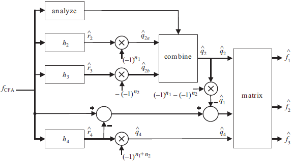
By tracing the demosaicking steps described in the figure and omitting any multiplications involving a constant operand, the number of multiplications S required to demosaic one image pixel is:
![]()
where filter h1 has order M1xM2, filter h2a has order N1xN2, filter h2b has order N1xN2 and the separable Gaussian filters hG1 and hG2 involved in the selection of weighting coefficients have orders P1 P2 and P2 P1 respectively. These filter orders are the only adjustable parameters that have any effect on computational complexity. The remaining adjustable parameters include the two-dimensional standard deviations (rG1, rG2) and the centering frequency parameter fm for the Gaussian filters hG1 and hG2. However, they do not change Gaussian filter orders and so they do not exert any influence on computational complexity. A systematic full search showed that (rG1, rG2) = (3.0, 1.0) is near optimal. Also recommendation in we set fm = 0.375 c/px.
The number of multiplications used by the algorithm can be reduced if we take into consideration filter proprieties. If we make use of the filter quadrantal symetry, the number of multiplications required to demosaic one pixel is:
![]()
If we make use of the fact tht the filters are separable than the number of computations required for demisaicking becomes:
![]()
The filter design training set and the demosaicking test set of color images consisted of subsets from the 24 Kodak photo-sampler images of size 512x768 that are widely used in the demosaicking literature. The figures below show the changes to objective demosaicking quality, measured by CMSE and S-CIELAB ΔE* ,as a function of computational complexity, measured by the number of multiplications, for one complete experiment with the greedy algorithm.
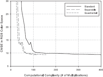
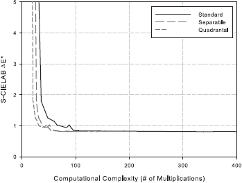
The experiment results confirm the tradeoff relationship between demosaicking quality and speed. The plots also show that the initial filter specifications can be simplified further without much degradation in objective quality. The configurations that best balance demosaicking quality and speed are the ones clustered about the transition from negligible changes to significant changes in CMSE and S-CIELAB ΔE*. Using the experiment results and favouring the least complex system possible, we identify the configuration [5 5 9 3 11 1] as a good choice. This corresponds to a 5x5 filter size for h1, a 9x3 least-squares filter h2a , a 3x9 least-squares filter h2b, an 11x1 Gaussian filter hG1 centered at (0.375, 0.0) c/px, and an 11x1 Gaussian filter hG2 centered at (0.0, 0.375) c/px. Both 1D Gaussian filters have a standard deviation of rG = rG1 = 3.0. During our own subjective evaluation, the demosaicked images produced by this configuration were perceived as being virtually identical to those from the more complex configurations. Of course, designers can choose whichever configuration gives their preferred tradeoff between quality and complexity.
The “quadrantal” and “separable” plots from the figure show that using quadrantally symmetric or separable filter approximations do not affect the tradeoff relationship. Quandrantal symmetry should definitely be used, whereas there is no advantage to use separability.
Some additional observations can be made about the filters themselves. In the first steps, the Gaussian filters hG1 and hG2 are reduced to one-dimensional filters. This is reasonable because at the centering frequencies (0.375, 0.0) c/px and (0.0, 0.375) c/px, there is usually little energy along the dimension not of interest (vertical for hG1 and horizontal for hG2) in the local frequency spectrum of the pixel undergoing demosaicking. Then, the order of h1 is reduced more quickly than the order of h2. Also, it appears the least-squares filter h1 prefers a square kernel, while the kernels for least-squares filters h2a and h2b can be made significantly rectangular.
The entire experiment was repeated by assigning different subsets of the Kodak dataset as the training and test sets. This included trials where the training set and test set were identical. In every case we observe the same tradeoff relationship reported by the figure. The sequences of chosen configurations do differ amongst the different setups. However, some configurations are consistently chosen at the same iteration. In fact, the identified configuration recommended earlier is one such configuration.