Course notes ELG 7187C - Behavioral Modeling

Developing the system requirements - an overview

The development of requirements is an important phase during system development. The course SEG-3101 covers the aspects of software requirements analysis in more details << C see my course notes from 2010 for more details >>. After requirements illicitation, there are normally several phases of requirements modeling and analysis at different levels, such as the following:

• Domain analysis: To identify the objects and actors within the environment of the system to be built, as well as the components of the projected system. To describe their properties, interactions and behavior aspects at an abstract level. An overview of a methodology for doing this is given in the SEG-2106 course notes - see also the hotel example.
• Goal-oriented modeling: Goals for the system must be defined and analysed. There are normally conflicts between different requirements that must be resolved. One should distinguish between functional goals (requirements) and non-functional goals ( non-functional requirements).
  • << C for more details, see SEG-3101 (goal modeling (first 17 pages), functional modeling, non-functional modeling). The book by Lamsweerde gives a good explanation of these concepts (Axel van Lamsweerde, Requirements Engineering: From System Goals to UML Models to Software Specifications, Wiley, 2009) >>
  • While functional requirements are normally clear-cut - such that it is possible to determine whether a given system satisfies them or not, non-functional requirements are often not so well defined; they are sometimes called "soft-goals". In view of expressing the trade-offs and desired priorities for the different non-functional properties of the system to be built, people have developed the so-called Goal-Oriented Requirement Language (GRL) C, which is being standardized by the ITU as part of the so-called User Requirements Notation (URN C ). << See also slides by D. Amyot (intro to GRL and UCM) and SEG-3101 course notes (starting page 18) >>
• Structural modeling: The domain model deals largely with structural issues. One normally uses Class Diagrams to represent such issues.We consider here the notation of UML Class Diagrams (see "Classes" C in the UML superstructure document).
• Behavioral modeling: R The dynamic behavior of a system with or without the external actors, or components of the system are often represented by state machine models or activity diagrams. States and activities (or actions) are complementary concepts and they are explicitly or implicitly shown by most of the modeling paradigmes. An introduction to the modeling with states and actions is given below.
  • Communication paradigms: The dynamic behavior of a system is defined in terms of its communication with its environment. Similarly, the dynamic behavior of system components is defined in terms of the interactions between these components. It is important to identify the actors (users) and system components that participate in these interactions. Also different types of interactions are considered by the different modeling paradigms that are used by different specification languages. There are essentially the following types of communication primitives (for details, see below):
    • rendezvous interactions
    • input-output interactions (which may contain data objects as parameters):
      • (a) with direct coupling of input and output transitions, and
      • (b) with message passing (implying some delay between output and subsequent consumption as input by another component)
    • procedure calls, which can be realized by the exchange of two messages between the client and the server: a call request message followed by a message returning the results (or indicating the termination of the server's actions).
    • shared variables: one particular scheme of using variables, is following an input-output approach. A shared variable can be written by one actor (output for that actor), and can be read by other actors (input for those actors)
  • Actors, components, resources: this aspect is not thought through very well in the above notations. Components and resources are important for performance considerations. See chapter on Performance Modeling.
  • Assuptions and guarantees: When defining the requirements that must be satisfied by a system within its environment, or by a system component within the environment of the other system components, it is important to consider the assumptions that can be made about the behavior of the environment of the component in question. One has to consider requirements that are structured in the following form: If "such and such assumptions are satisfied by the environment" then the behavior of the specified system component will "satisfy such and such guarantees"; the assumptions imply the guarantees. These considerations are important for component re-use, when one wants to decide whether an implementation satisfying requirements R1 can be used where the system design requires an implementation satisfying requirements R2 (see requirements with assumptions and guarantees).

Introduction to state-oriented modeling

See course notes for SEG-2106 , Chapter 2 R and the Coffee Machine example R

Workflow modeling: This is a particular type of behavioral modeling. Usually, notations similar to UML Activity Diagrams are used (see "Activities" C in the UML superstructure document). Another notation, Use Case Maps C (UCMs, part of the ITU URN standardization) has a very similar semantics. Both notations define in which order the activities mentioned within a diagram may be executed. The main differences between these notations are (i) UCMs look more informal, (ii) UCMs allow more flexibility for defining the different system components that are responsible for the different activities performed, and (iii) Activity Diagrams allow (but not UCMs) the specification of the classes of objects exchanged as input or output between the different activities (data flow). Here is a comparison. There is also several other languages that represent extensions of the concepts in Activity diagrams, such as Business Process Modelling Notation (BPMN) C , a language that uses most of the concepts of Activity Diagrams (an overview of the language can be found in Section 7 of the current definition C ).

• Note: The semantics of Activity Diagrams and related notations is strongly influenced (if not based on) Petri nets. Petri nets are formal models of dynamic behavior (published by Petri in his PhD thesis, 1962). See below for more details.
• << Here is an industrial example of supply chain management, see use cases, architecture, usage scenarios >>
• More on UCMs: C A tutorial introduction to GRL and UCM is given in ComNet'03. The tool jUCMNav supports both GRL and UCMs. << Another example of supply chain management is discussed in MCeTech'05 . See in particular Figure 4 for the GRL notation for dependencies between the goals of different "actors" (customers, retailers, warehouses, manufacturers); a comparison between different architectures is given in Section IV under the title "evolution", however, this topic is not clearly elaborated >> 

Different categories of state-transition models

Chapter 2 of the course SEG-2106 concentrates on state-transition models with a finite number of states. Often this is too limiting and one uses so-called extended state-transition models where the state includes the value of state variables and interactions may include data parameters. One needs more powerful specification formalisms for defining their behavior. Here is an overview.

Models of communicating state machines

For an introduction to the issues, see course notes for SEG-2106 , Chapter 3 R

Constructing a global model - "reachability analysis" R

Examples: Hotel, LTSA examples from SEG-2016, alternating bit protocol, assignment-1 (2012) (Activity diagram), assignment-2 (2012)

Petri nets

• While a single state machine has no concurrency, a single Petri net model includes in general concurrent behaviors. A Petri net contains in general several tokens that reside at different places ( a place is similar to a state), and the state of the Petri net is defined by the distribution of tokens over the places. At each moment in time, several transitions may be enabled (depending on the distribution of tokens) and they may be executed concurrently.
• A single Petri net model often contains several interconnected parts, where each part, in a sense, represents the behavior of a system component. Some of the tokens may represent a message that is in transit from one system component to another.
• See here R for more details.

Comparison of different formalisms

To compare these different formalisms, it is interesting to consider an example system specified in these different formalism. We may consider the alternating bit protocol (ABP) for this purpose. As an introduction to this example, see my paper on Finite State Description of Communication Protocols of 1978, which contains a Sender and a Receiver component that communicate with one another and with respective user components. The paper uses a kind of IOA approach were the communication medium is represented as a separate system component.

A different model for the ABP using only 3 states plus a variable containing the alternating bit is described in my paper of 1977 A. This is an example of using the extended IOA modeling approach. The verification of properties becomes more complex, because the finite-state-reachability is not sufficient to prove interesting properties, one also has to consider the content of the variables and consider assertions involving these variables.

Question: How could one describe the protocol with the FSM formalism (with asynchronous communication) ?

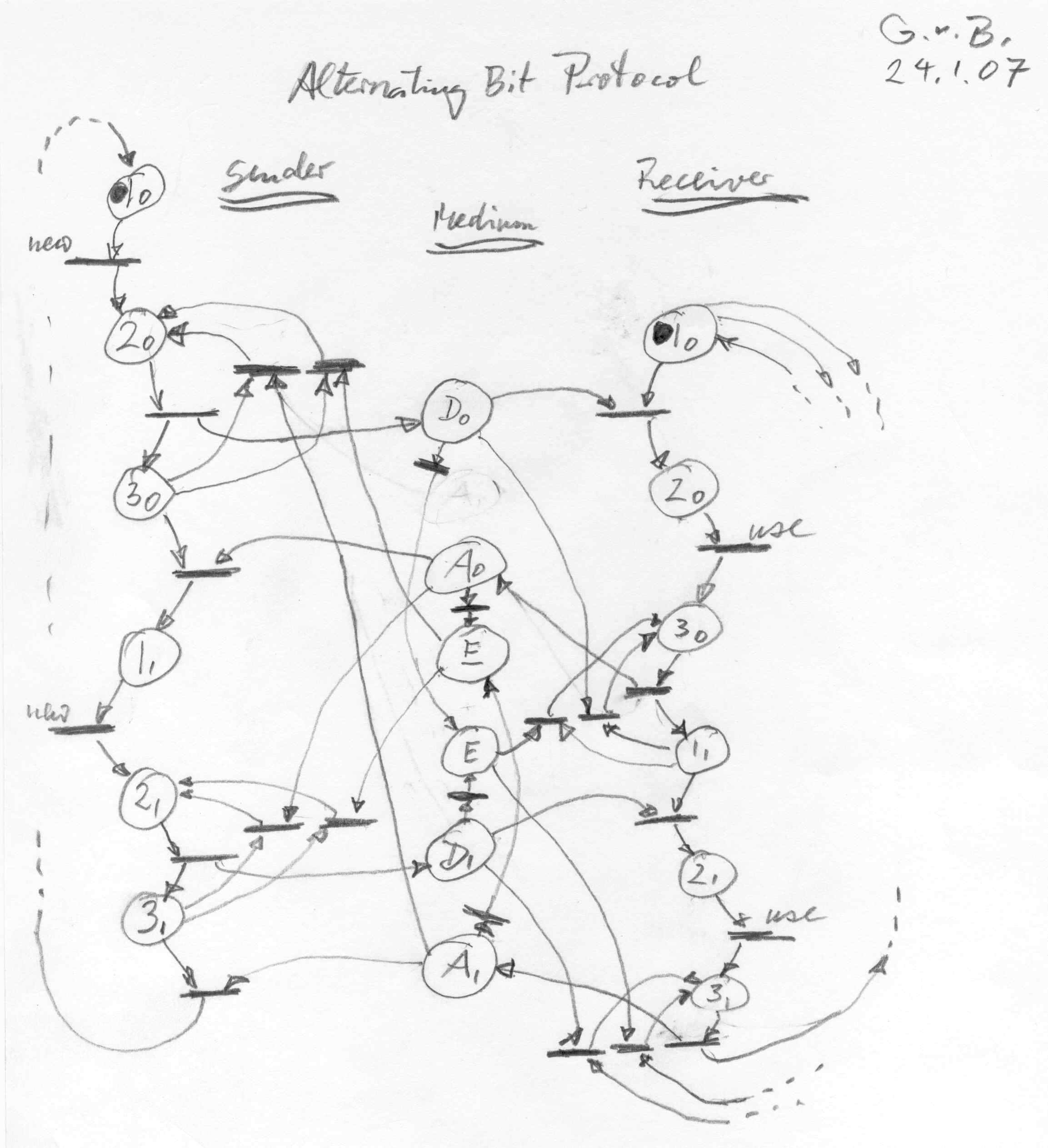
And how could the protocol be modelled with Petri nets ? (Note: There is a "pattern" to represent FSM states in Petri nets, and there is a "pattern" to represent messages in transit between different components - see Figure (e) on Petri Net Page). Here is a diagram showing the alternating bit protocol as a Petri net R. (Note: in this example, the whole system is modeled as a single Petri net).

Criteria for comparison

• Ease of modeling
• Ease of deriving properties automatically

Complementary readings

• Earlier course notes - Powerpoint slides: CourseNotes2 on transition systems; CourseNotes3 on FSM models; Concordia-Tutorial (the part entitled "Preliminaries") covering all these points, but only very shortly.
• The following papers of mine deal with the topic:
  • Finite state description of protocols A-R (1978): explains reachability analysis using the Alternating Bit Protocol as example
  • Unified method ... A (1977): presents an extended FSM modeling approach and compares it with the FSM approach in the above paper.
  • Protocol specification for OSI A (1990): provides an overview of formal and informal methods for protocol specification, verification and implementatio

Created in 2007; last update: January 29, 2013