Course notes for SEG-2106
One sometimes makes the distinction between:
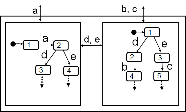
The composite structure of a system can be described by informal structure diagrams (as I often use for my explanations - see for instance the Coffee Machine example - note: these diagrams represent closed systems - the user is included) or with UML Composite Structure diagrams (see example - Note: this diagram represents an open system). In UML, a port (interface) may be an In-Port (only accepting inputs) or an Out-Port (only supporting the production of outputs), or both. The UML Composite Structure diagram also may contain connectors that connect ports of sub-components or which connect an external port of the system with ports of a sub-component which effectively realizes the external port of the system. For each port, one can define the set of interactions supported. Clearly, the connectors should be such that the interconnected ports are compatible as far as the exchanged interactions are concerned.
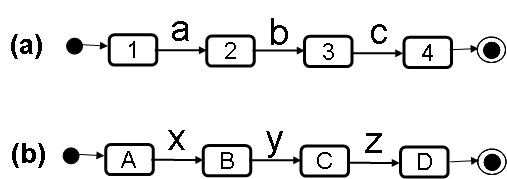
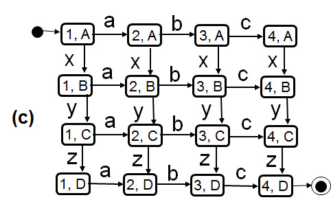
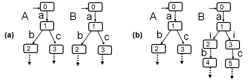
Concurrent processes give rise to a large number of possible interaction sequences because the execution of sequences of the different processes may be interleaved in many ways. In the case of independent concurrency, as defined by parallel regions of UML State diagrams, one assumes by default that there is no interrelationship between the concurrent processes (no communication, no shared resources, nor shared variables). This has the advantage, that the behavior of each process can be analysed independently of the other processes. However, the number of possible overall execution sequences is the largest, because the actions of the different processes may be interleaved arbitrarily in the global execution trace. An example is shown in the following diagrams, where (a) and (b) represent two independent processes, defined in the form of LTSs, and (c) shows the resulting global behavior (also in the form of an LTS). In this example, one assumes that the LTS transitions take no time, therefore the execution of two transitions of two different LTSs can be assumed to be sequential, one after the other, and when the LTS are independent and two transitions of different LTSs are enabled, then their order of execution is not determined; there is therefore some non-determinism introduced by this form of concurrency. This is called interleaving semantics. The situation becomes more complex when one assumes that transitions take some time; then one must consider the case that two transitions are in the process of being performed at the same time; one may describe such situations by considering for each transition of the original model, two sub-transitions and an intermediate state: the first sub-transition corresponds to the beginning of the transition, and the second one to its end. The intermediate state represents the state of the LTS when the transition is taking place; (this will not be considered further in this course).
We consider in the following that several state machines operate concurrently, but not independently (as in concurrent regions of State Charts). We consider that the behavior of one machine is influenced by the behavior of the other machines. There are different ways that these dependencies can be modelled. The most important paradigms for modeling communication were discussed in the previous chapter. In this course we only consider rendezvous communication, procedure call and asynchronous message passing.
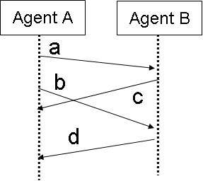
We now consider an example where there is some communication/collaboration between two different agents (possibly located on different sites). We first consider a global view (which may correspond to the functional model elaborated during the requirements phase). Again, we show two different models, one UML State diagram (a) and one UML Activity diagram (b), and these two models are equivalent (have the same "meaning" - semantics). Actions a and b are performed by agent A and actions c and d are performed by agent B, and the order in which these actions should be performed is defined by the following diagrams: We note that the ordering constraints defined by these diagrams imply that there is probably some data produced by actions b and some data produced by action c that is required for action d.
.jpg)
.jpg)
.jpg)
In order to understand the meaning of these two diagrams, we consider trace semantics, that is, we ask the question: What are the valid traces (that is, sequences of action executions) ? - Our intuitive understanding of the above diagrams should lead us to the following set of valid traces: <a, b, c, d>, <a, c, b, d>, and <c, a, b, d>. These are also the traces of the LTS shown above as diagram (c). Therefore this LTS has the same meaning (semantics) as the two UML diagrams above.
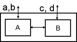
All three diagrams present the functional behavior from a global view; the fact that two different agents are involved is not explicitely modelled here. Now we consider a particular system structure consisting of two components A and B, each being responsible for a subset of the interactions, as shown in the following diagram.
The diagram shows that there are two interfaces, realized by component A and B, respectively. A performs the interactions a and b, while B performs the interactions c and d. The type of interactions between the two components is not specified here.
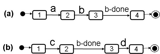
In this subsection, we consider rendezvous communication between the two components and with the system environment. We have noticed from the understanding of the global system behavior described above, that agent B has to wait that agent A has completed its action b, before it could start with its action d. Therefore we may introduce a rendezvous interaction between the two agents with the name b-done which should be performed by B before starting the action d and which should be enabled by A as soon as it has finished with its b action.
We can start out with a behavior definition for A and B obtained by projecting (see concept explained in Chapter 1) the global behavior (diagram (c) above) onto the set of interactions each agent is involved in. This leads to the following:
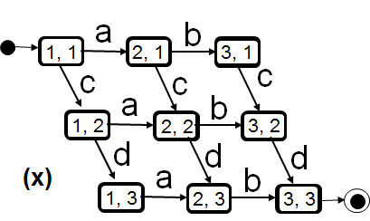
If we adopt these behaviors for the two agents (without any communication between the two, see diagrams (ax) and (bx) below), we obtain the global behavior (of independent concurrency) shown in diagram (x) below. This behavior includes all the traces defined by the given system behavior in diagram (c) above, but it also contains other traces, for instance <c, d, a, b>, which are not valid according to the given system requirement. Whe therefore have to find a behavior of the two agents that is more restrictive.
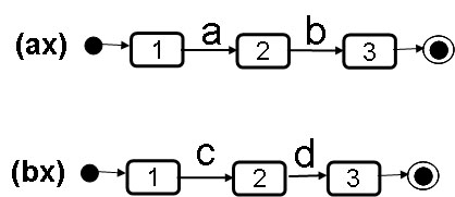
One way to introduce restrictions is by introducing synchronization points (rendezvous interactions) between the two behaviors. Following this approach, we may add the rendezvous b-done between the two agents, by defining the following traces for the behaviors of the two agents (both have a behavior represented by a single trace): behavior of Agent A = { <a, b, b-done> }; behavior of Agent B = { c, <b-done, d> }. These behaviors are represented by the diagrams (a) and (b) below:
This appears to be a reasonable design process for the behavior of the two agents, but we have to verify this design. This means, we have to deduce the global behavior obtained by the composition of these two agents and compare this behavior with the required behavior (shown in the diagram (c) above). This means, we have to find methods for solving the following two problems:
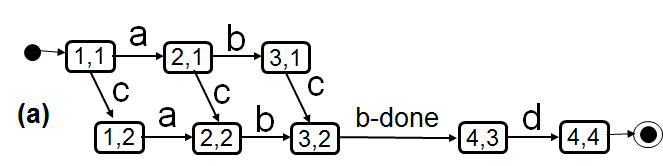
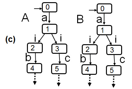
This problem, for LTS specifications, can be solved by constructing the so-called product of the components. This product behavior is again an LTS where each state of this global LTS identifies the states of the two component LTSs. As an example, we show how the product of the two agent LTS specifications can be obtained. The initial state is (1, 1) - both agents are in their initial state. In this state, either agent A may do an a transition, or agent B may do a c transition (which leads us into two different states (2, 1) or (1, 2), respectively; and so on. The resulting global LTS is shown below as diagram (a). If one explores systematically all possible states and transitions of the global product, the process of constructing the product behavior is called reachability analysis (finding all states and transitions of the product behavior that can be reached from the initial state); note that some global states, such as (1,4) in this example, are not reachable (and therefore can never occur).
We would be happy if the behavior of this global LTS would be the same as the one defined system behavior in diagram (c) above. It is not the same because of the following reasons:
What criteria should be used for comparing the global behavior of the communicating components with the given required system behavior? - We have to compare two behaviors: (a) the global behavior of the communicating components (the more detailed model), and (b) the global system behavior given as the requirements (the more abstract model). Under which criteria can we say that the detailed model satisfies the requirements of the abstract model ? - First, we make abstraction from the internal interaction in the model (a) (because they are not included in the abstract model (b)). Then we consider two criteria:
It is important to note that the component behavior of several components, after having projected out the internal rendezvous interactions between the different components, often leads to global behaviors that are non-deterministic. This means that an observer of the system, observing through the system interfaces only, may not know in which state the system is at some particular point during the execution of a trace.
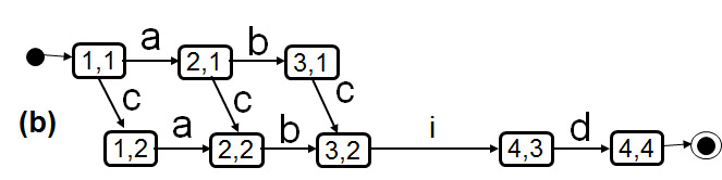
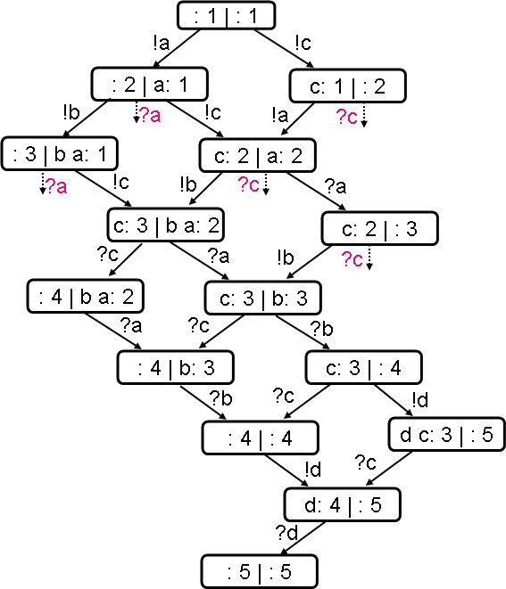
Sometimes one uses non-deterministic behavior to model the fact that a component can make the choice between two alternatives. A well-known simple example is the following: In the system described by the two agents in diagram (a) above, there are two choices, but it is not defined which agents makes the choice, or whether both parties are involved in the choice, or whether there may be a random choice (performed by some third party). In the system shown in diagram (b), it is quite clear that agent B makes the choice between the two alternatives when it choses between the two "internal" transitions labelled i. These are spontaneous transitions without any interaction with the environment of the agent. One can say that the Agent B is active in this choice while Agent A is passive (accepting any alternative). If two active agents are involved in a choice (see diagram (c)), they may lead the system into a deadlock if they have chosen different alternatives during their internal choice process.
Here we consider that the components of the system communicate by message passing, that is, for each passed message, there are two events: the sending event performed by the source component, and the receiving event performed by the destination component. The message passing delay is assumed to be unknown. In the following we assume that messages are not lost.
Note: Often one assumes that the destination component has a queue in which received messages are stored before they are consumed by the defined behavior of the destination component. Sometimes, separate queues are assumed for each different source component. Sometimes one assumes that the behavior of the receiving component can determine in which order received messages will be consumed (processed). In SDL, the SAVE construct is used for this purpose, and in UML one talks about deferred events (see UML "Unexpected event reception"). This is sometimes very useful, but will not be further discussed in this course. <<graduate course: message queuing>> In the following, we assume that the incoming messages are placed in a FIFO queue before being processed by the state machine.
In the following, we discuss again the abcd-Example. As before, we assume that the actions a and b, and c and d are performed agents A and B, respectively, but we also assume that the results of all these actions are shared with the other agent (similar as the result of action b in our earlier example was shared with Agent B). This sharing is performed by sending a message to the other agent. This leads us to consider the following sequence diagram describing the behavior of the two components. We take this sequence diagram as the global system requirement, that is, the two components should realize the following sequence diagram.
As in the section above on rendezvous communication, we would like again to somehow derive the behavior of the two agents in such a way that their communication through the exchange of a, b, c, and d messages leads to a global behavior of the sequence diagramme above, which can be considered a use case.
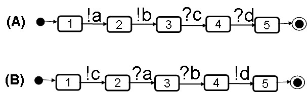
A typical design method (for this purpose) is to look at the sequence of actions performed by a given agent according to the given sequence diagrams describing the use cases. In this example, we only have the use case above. This sequence diagram shows for agent A the sequence of actions as follows: <!a, !b, ?c, ?d>, where the symbol "!" means sending and the symbol "?" means receiving. Similarly, the behavior of Agent B is predicted as following the trace <!c, ?a, ?b, !d>. These two behaviors are shown as state machines below.
The next step in our design work of defining the behaviors of the two agents is the verification that the behaviors proposed above are valid. Again, we have the two problems: (1) How to determine the global behavior that results from the given behavior of the components, and (2) how to compare the derived global behavior with the system behavior given as requirement. In the following we discuss the first problem.
As we did in the case where we discussed this example with rendezvous interactions, we should verify that the proposed behavior of the two components, when they are composed according to the system architecture shown above (but now communicating by asynchronous message exchanges), conforms to the behavior defined by the sequence diagram shown above. For this purpose, we do again a reachability analysis to obtain the behavior of the composed system.
Reachability analysis for components communicating by asynchronous messages is more complex than reachability analysis for state machines communicating by rendezvous (as discussed above). While with rendezvous communication, there is never any message is transit; a state of the global system is defined by the states of all its components. However, in the case of components communicating by message passing, the fact that a message is in transit has an impact on the future behavior of the global system, and therefore such messages must be included in the description of the state of the global system.
The dotted arrows with the red interaction labels indicate that in these states, there is a non-specified reception. This is the situation where for the next message to be received by an agent (already in the input queue in front of the ":" symbol) there is no transition to consume this message in the current state. For instance, in the global state " : 2 | a: 1 ", the message a is waiting to be received, but Agent B in state 1 has no transition to receive such a message. The presence of global states in the reachability graph with non-specified receptions indicates that the behavior of the communicating agents are not compatible with one another. This is usually a design error. For our example, the reachability graph above therefore shows that the design of the behaviors for the agents A and B, as defined by the diagrams above, is flawed. <<graduate course: non-specified reception>>
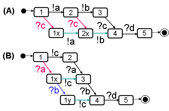
Since the transitions included in the agent behaviors above are all necessary in order to realize the sequence diagram above (that defines the desired behavior of the overall system), the only way to improve our design is by adding transitions to the agent behaviors. In fact, by looking at the unspecified receptions high-lighted in red in the above diagram, we see that Agent A should be able to receive message c in states 1 and 2, and Agent B should be able to receive message a in state 1. This is indicated in red in the extended agent behaviors shown in diagrams (A) and (B) below. Note: We also have to choose appropriate next states for these transitions - I do not know any methodology for this.
The reason for the non-specified receptions encountered in our example is the fact that the message transmission delay may be much shorter than assumed in the above sequence diagram, and therefore a transmitted message may already be received in the initial state. Since Agent A may send two messages, a and b, very early, it could happen that both of these message would be received by Agent B before it had sent its message c. For this reason, we have included the additional blue transition in the behavior definition of Agent B below. We note that we have also included several transitions indicated in green in the extended agent behaviors. The design of these transitions was made in order to produce the message sending actions required by our initial sequence diagram.
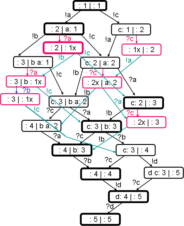
We should now verify our extended design and check what kind of global system behavior it entails. Doing the reachability analysis again, we obtain the graph shown above (on the right). The colors in the reachability graph correspond to the colors of the transitions in the agent behavior. For each state with a non-specified reception in the earlier reachability graph, the new graph includes a new global state (in red), and the blue transition of Agent B also leads to an additional state. As expected, the new reachability graph includes the earlier one (since the revision of the agent behaviors only included additional transitions, no transitions were removed).
We notice that the new graph has no non-specified receptions; this means that the behaviors of the two agents are compatible (there is no internal problem considering the system as a black box). This corresponds to internal consistency of the system design. However, verification also includes checking that the resulting behavior of the system conforms to the desired behavior of the system (which was defined in terms of the sequence diagram above) - see next subsection.
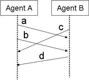
The sequence diagram defining the requirements is copied below (left diagram). What is the meaning of such a sequence diagram ? - <<graduate course: an answer was explained in 1978 in a paper by Leslie Lamport talking about "logical time" and the partial order between events>>
The fact that certain events in the sequence diagram are not ordered, leads to the different execution sequences shown in our first reachability graph. The different paths through that graph are all consistent with our original sequence diagram (blow on the left). We note, however, that the execution sequence shown in the extended reachability graph (above, on the right) in the form of fat state symbols is not compatible with this sequence diagram; it corresponds rather to the sequence diagram shown below on the right (which is called a scenario implied by the original sequence diagram on the left). The difference is the order between the reception of a and the sending of c by Agent B.
Conclusion: We see that the behavior of (A) and (B) as modified with the additional transitions in color (required to avoid non-specified receptions) gives rise to new execution sequences that are incompatible with the original sequence diagram (on the left). Please note that this is "normal".
The fact that, in many cases, a given sequence diagram cannot be realised alone, but any design of components that realizes the diagram necessarily also realizes other sequence diagrams is an interesting observation. The other sequence diagrams that necessarily are also realized by the distributed system are called implied scenarios (they are implied by the scenario originally given) <<graduate course: they were first described in a paper by Alur et al.>>.
You can find LTSA models of the abcd-Example in the files abcd-Example - rendezvous and abcd-Example - message passing.
Here is another example of reachability analysis (from the course notes of 2010)
If the reachability analysis identifies design flaws, the behavior specification of the system should be revised. Here are some suggestions of possible strategies for such revisions.