
This page describes in detail the luma-chroma demultiplexing formulation for demosaicking of signals sampled with the diagonal stripe CFA of section 7.3.3.2, along with the results of the least-squares filter design, organized as shown below. Software is provided to allow these results to be reproduced.
Geometric structure of the Diagonal stripe color-filter array
Formation and representation of the Diagonal stripe CFA image
Least-squares filter design for CFA signal demultiplexing
Least-squares luma-chroma demultiplexing (LSLCD) algorithm results for the stripe pattern
LSLCD optimization - quality vs complexity
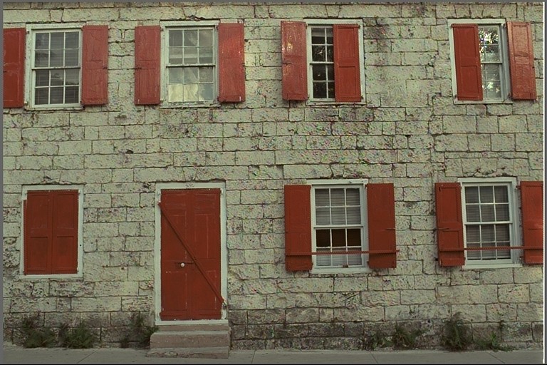
The geometric structure of the diagonal stripe pattern is similar to that presented in the sample below:

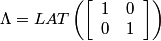
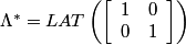
The Diagonal stripe pattern is regular and periodic. It lies on an integer lattice Λ = ℤ2. The horizontal and vertical sampling spaces in this samping structure are equal. The distance between them is X, used as the unit of length, pixel height (px).
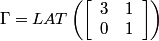
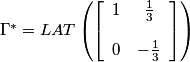
The Diagonal stripe structure has three classes corresponding to the red (R), green (G) and blue (B) filters. The origin of the set is at the upper left corner with a red sample. The red, green and blue pattern is repeated periodically. The nearest same-color sample is found on the lower right corner of each sample. One period of the Stripe pattern determined by the sublattice Γ is indicated by the bold contour in the upper left corner.
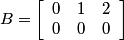
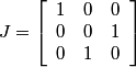
Following the chapter's theory, one can describe the Diagonal stripe pattern using matrices.
 ,
,
 .
.
 .
.
 .
.
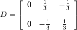
In the frequency domain the Diagonal stipe pattern has the following characteristics:
 ,
,
 .
.
 .
.
Considering the choices made above, we obtain the following :
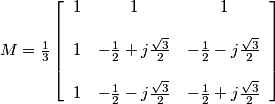 .
.
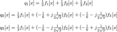 .
.
Here, we see that q2[x]and q3[x] are complex and q3[x] = q2*[x].
The inverse transformation recovers the original components using the matrix M-1
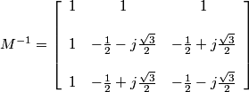 .
.
In the frequency domain FCFA, becomes:
 .
.
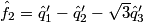
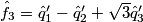
The use of complex signals can be avoided by expressing the modulation as a quadrature modulation of real signals. Rather than considering the two modulated signals:

we can consider the equivalent real, quadrature modulated signals:

where

and
 .
.
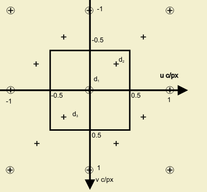
One period of the two-dimensional power density spectrum of a sample CFA image with the diagonal stripe CFA structure is shown below.
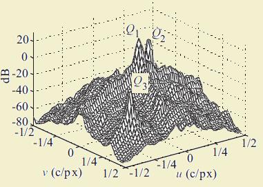
The three different components are identified in the figure.
The idea behind demosaicking algorithms based on the frequency-domain representation is to extract the luma and modulated chrominance components from the CFA signal using spatial filters and then to transform the demodulated chrominance components to the desired tristimulus values.
In the case of the Diagonal stripe pattern, the demosaicking algorithm is straightforward:
1. Filter fCFA with a complex bandpass filter h2
centered at frequency ![]() to extract
to extract  , and shift it to baseband to estimate
 .
.
2. Estimate the luma component

3. Estimate 
4. Estimate the RGB components  from
from 
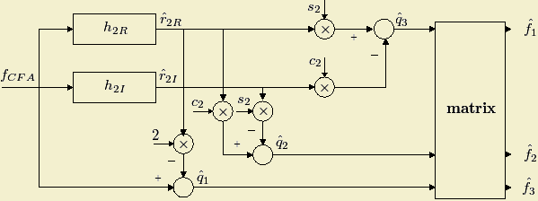
In practice, the input and output signals are real, and the complex operations above can be expanded to obtain the real version of the algorithm:


The block diagram of the demultiplexing algorithm for the stripe structure is represented below:
The LSLCD algorithm for the diagonal stripe structure follows exactly the approach in the chapter.
An example of designed filters can be seen here.
For our testing, we used different training sets:
A full list of results for the 24 Kodak images can be found here.
The table below shows the LSLCD algorithm results for the first 3 Kodak images. The training set chosen here is all the 24 Kodak images. :
| No. | Thumb | Original | LSLCD |
| 1 |  |
TIFF | TIFF
36.87 |
| 2 |  |
TIFF | TIFF
38.93 |
| 3 |  |
TIFF | TIFF
39.46 |
The quality of the demultiplexed image and the complexity of the filters used in the algorithm are directly related. The quality versus complexity plot for the diagonal stripe pattern is below. The optimization algorithm details and the related observations can be found here.
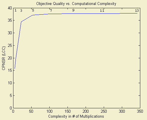
The recommended filter size is 5x5.
Lslcd algorithm computations: Stripe_LSLCD
Metrics: CPSNR calculator.