Chapter 9 Random Field Models
MATLAB code for figures and examples
- Fig. 9.1 Illustration of three realizations of a two-dimensional color random field.
- MATLAB script: mdsp_web_random_randomField.m
- Output preview: fig9.1_1.png; fig9.1_2.png; fig9.1_3.png
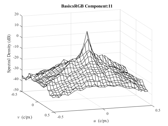
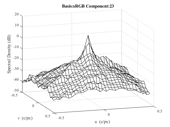
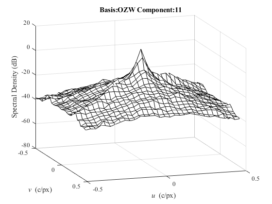
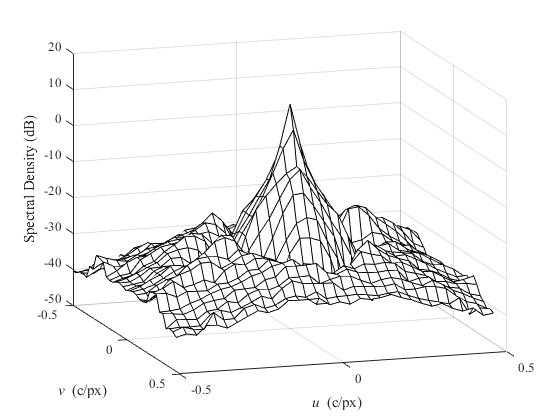
- Fig. 9.3-9.4 Elements of spectral density matrix in dB for Kodak motorcycles image (#5) using different bases of color space.
- MATLAB script: mdsp_web_random_color_spectra.m
- Output preview:
- Fig. 9.3 sRGB basis: Uncomment A_sRGB2B = eye(3); bas = 'sRGB'. fig9.3a.png; fig9.3b.png; fig9.3c.png; fig9.3d.png; fig9.3e.png; fig9.3f.png
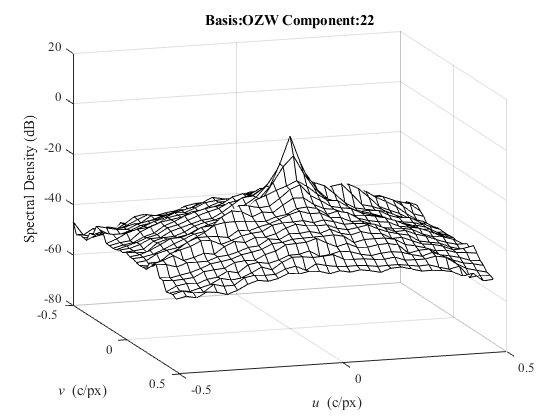
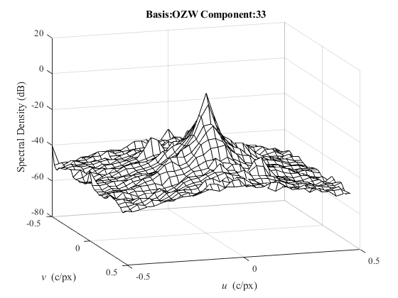
- Fig. 9.4 OZW basis: Uncomment A_sRGB2B = A_XYZtoOZW*inv(A_XYZtosRGB); bas = 'OZW'. fig9.4a.png; fig9.4b.png; fig9.4c.png; fig9.4d.png; fig9.4e.png; fig9.4f.png
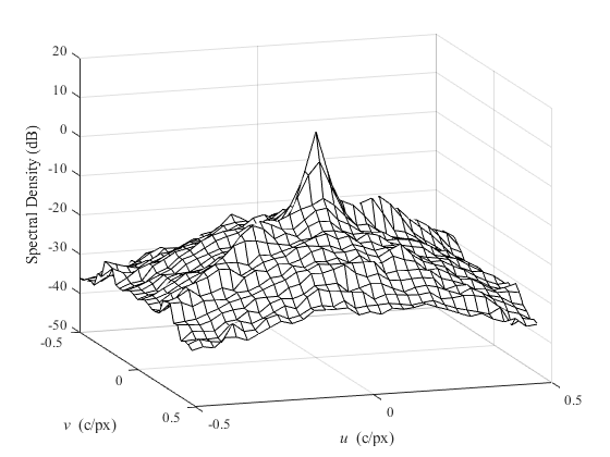
- Fig. 9.5-9.6 Elements of spectral density matrix in dB for Kodak motorcycles image (#5) using Zhang and Wandell OZW opponent basis of color space, where the components O2 and O3 have undergone a lowpass filtering operation.
- MATLAB script: mdsp_web_random_OZW_filt.m
- Output preview:
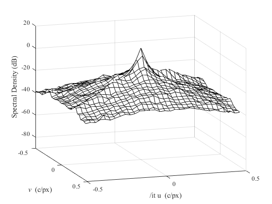
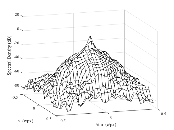
- Fig. 9.5 OZW basis: fig9.5a.png; fig9.5b.png; fig9.5c.png; fig9.5d.png; fig9.5e.png; fig9.5f.png
- Fig. 9.6 RGB basis: fig9.6a.png; fig9.6b.png; fig9.6c.png; fig9.6d.png; fig9.6e.png; fig9.6f.png