Chapter 10 Analysis and Design of Multidimensional FIR Filters
MATLAB code for figures and examples
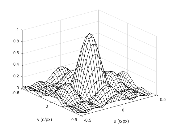
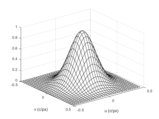
- Example 10.1 — Fig. 10.2-10.4 Frequency response of a moving average filter with L = 2 and Gaussian filter. Result when applied to image Barbara.
- MATLAB script: mdsp_web_design_FIRfilt_design_examp.m
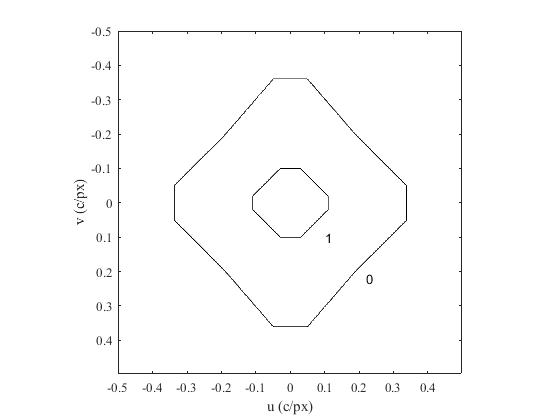
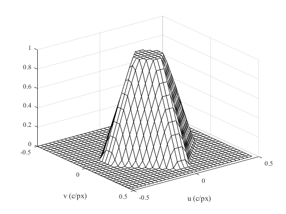
- Fig. 10.2 (a) Moving average filter, contour plot. Output preview: fig10.2a.png
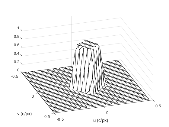
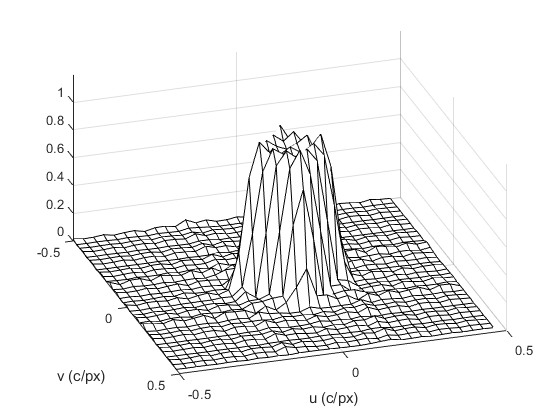
- Fig. 10.2 (b) Moving average filter, perspective plot. Output preview: fig10.2b.png
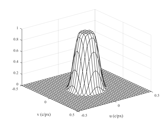
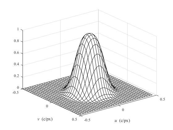
- Fig. 10.3 (a) Gaussian filter, contour plot. Output preview: fig10.3a.png
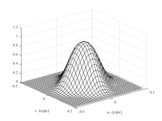
- Fig. 10.3 (b) Gaussian filter, perspective plot. Output preview: fig10.3b.png
- Fig. 10.4 (a) Barbara image filtered with moving average filter. Output preview: fig10.4a.jpg
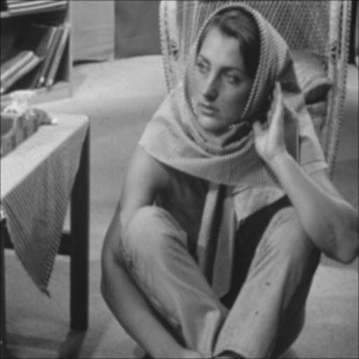
- Fig. 10.4 (b) Barbara image filtered with Gaussian filter. Output preview: fig10.4b.jpg
- Example 10.2 — Fig. 10.5-10.7 Frequency response of Gaussian band-stop filter with center frequency (150, -86) c/ph. Applied to image Barbara.
- MATLAB script: mdsp_web_design_gaussian_band_stop.m
- Fig. 10.5 Band-stop filter, perspective plot. Output preview: fig10.5.png
- Fig. 10.6 Barbara image filtered with band-stop filter. Output preview: fig10.6.jpg
- Fig. 10.7 Close-up of knee filtered with band-stop filter.Left original; right filtered. Output preview: fig10.7_left.jpg; fig10.7_right.jpg
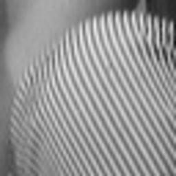
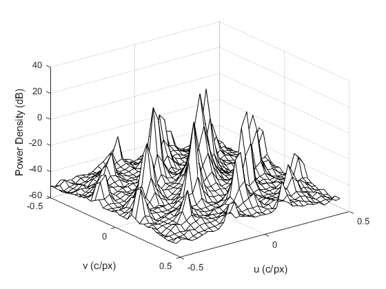
- Example 10.3 — Fig. 10.8-10.12 Filter a halftone image with a multi-band-stop filter. Input image, output image and spectra; points of the halftone interference pattern within one unit cell of the reciprocal lattice
- Fig. 10.8, 10.9, 10.11, 10.12 MATLAB script: mdsp_web_design_halftone_attenuate.m
- Fig. 10.10 MATLAB script: mdsp_web_design_halftone_lattice.m
- Fig. 10.8 Input preview: fig10.8.jpg
- Fig. 10.9 Spectrum of input image. Output preview: fig10.9.png
- Fig. 10.10 Points of halftone interference pattern. Output preview: fig10.10.png
- Fig. 10.11 (a) Spectrum of input image. Output preview: fig10.11a.png
- Fig. 10.11 (b) Spectrum of output image. Output preview: fig10.11b.png
- Fig. 10.12 Filtered halftone image. Output preview: fig10.12.jpg
- Fig. 10.13 Radial profile of three circularly symmetric ideal responses with 3dB radial frequency cutoff of 0.125 c/px.
- MATLAB script: mdsp_web_design_ideal_circ_resp.m
- Fig. 10.13 (b) Step transition. Output preview: fig10.13b.png
- Fig. 10.13 (c) Linear transition. Output preview: fig10.13c.png
- Fig. 10.13 (d) Raised-cosine transition. Output preview: fig10.13d.png
- Fig. 10.14 Boundaries of polygonal pass and stop bands of an example ideal lowpass frequency response; perspective view of the ideal frequency response with planar transition band.
- MATLAB script:mdsp_web_design_ideal_polygonal_response.m
- (a) Boundaries of polygonal pass and stop bands. Output preview: fig10.14a.png
- (b) Perspective view of the ideal frequency response. Output preview: fig10.14b.png
- Fig. 10.15, 10.16 Frequency response of approximation to ideal circularly symmetric lowpass filter with -3dB point at radial frequency 0.125 c/px using the window method. Set L and W as indicated in the figure caption; result of filtering the Barbara image with this filter.
- MATLAB script: mdsp_web_design_circular_window_FIR.m
- Fig. 10.15 (a) Size 13 x 13 (W = 0:171) contour plot. Output preview: fig10.15a.png
- Fig. 10.15 (b) Size 13 x 13 (W = 0:171) perspective plot. Output preview: fig10.15b.png
- Fig. 10.15 (c) Size 21 x 21 (W = 0:1498) contour plot. Output preview: fig10.15c.png
- Fig. 10.15 (d) Size 21 x 21 (W = 0:1498) perspective plot. Output preview: fig10.15d.png
- Fig. 10.15 (e) Size 41 x 41 (W = 0:1366) contour plot. Output preview: fig10.15e.png
- Fig. 10.15 (f) Size 41 x 41 (W = 0:1366) perspective plot. Output preview: fig10.15f.png
- Fig. 10.16 (a) Barbara image filtered with 13 x 13 filter. Output preview: fig10.16a.jpg
- Fig. 10.16 (b) Barbara image filtered with 41 x 41 filter. Output preview: fig10.16b.jpg
- Example 10.4 — Fig. 10.17 Least pth design for low-pass filter with polygonal specifications shown in Fig. 10.14.
- MATLAB script: mdsp_web_design_leastpth_polygonal.m
- Fig. 10.17 (a) Size 13 x 13 least pth design. Output preview: fig10.17a.png
- Fig. 10.17 (b) Size 13 x 13 window design. Output preview: fig10.17b.png
- Fig. 10.17 (c) Size 21 x 21 least pth design. Output preview: fig10.17c.png
- Fig. 10.17 (d) Size 21 x 21 window design. Output preview: fig10.17d.png
- Example 10.5 — Fig. 10.18, 10.19 Low-pass filter for halftone suppression; filtered image with and without equality constraints on the frequency response. Must uncomment filter_design_zp_con (line 29) or filter_design_zp_unc (line 30) depending on which is desired.
- MATLAB script: mdsp_web_design_halftone_lpf_constraints.m
- Fig. 10.18 (a) Ideal response. Output preview: fig10.18a.png
- Fig. 10.18 (b) Least pth design with no constraints. Output preview: fig10.18b.png
- Fig. 10.18 (c) Least pth design with constraints. Output preview: fig10.18c.png
- Fig. 10.19 (a) Halftone image filtered without constraints. Output preview: fig10.19a.jpg
- Fig. 10.19 (b) Halftone image filtered with constraints. Output preview: fig10.19b.jpg