Chapter 11 Changing the Sampling Structure of an Image
MATLAB code for figures and examples
- Example 11.1 — Fig. 11.1-11.3. Illustration of lattice and sublattice, and application to upsampling operation.
- Fig. 11.1 Plot a lattice with a sublattice.
- MATLAB script: mdsp_web_changesamp_plot_2D_lattice_sublattice.m
- Output preview: fig11.1.png
- Fig. 11.2 Upsampling in the frequency domain.
- MATLAB script: mdsp_web_changesamp_plot_2D_recip_lattice_sublattice.m
- Output preview: fig11.2.png
- Fig. 11.3 Illustration of unit cells of reciprocal lattices.
- MATLAB script: mdsp_web_changesamp_plot_2D_recip_sublattice_spect.m
- Output preview: fig11.3.png
- Example 11.2 — Fig. 11.5-11.7 Upsampling of rectangularly sampled signal by a factor of 4 in each dimension.
- Fig. 11.5 Frequency domain view.
- MATLAB script mdsp_web_changesamp_upsample16_spect.m
- Output preview: fig11.5.png
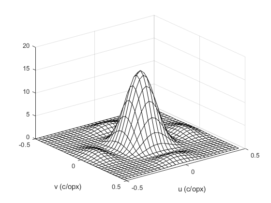
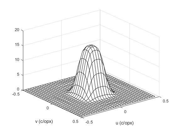
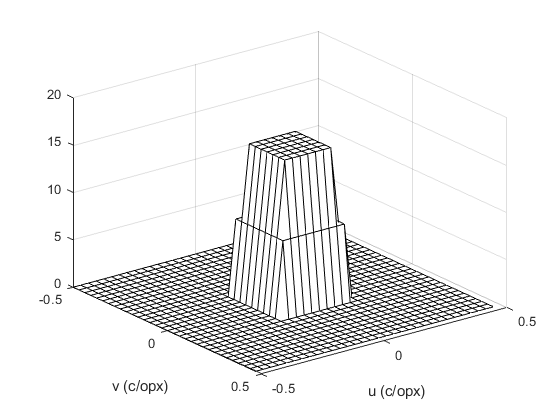
- Fig. 11.6 Perspective view of the frequency response of interpolation filters for 16:1 interpolation.
- MATLAB script: mdsp_web_changesamp_upsample16_filters.m
- Fig. 11.6 (a) Bilinear interpolator. Output preview: fig11.6a.png
- Fig. 11.6 (b) Bicubic interpolator. Output preview: fig11.6b.png
- Fig. 11.6 (c) Ideal response. Output preview: fig11.6c.png
- Fig. 11.6 (d) 29 x 29 least pth design. Output preview: fig11.6d.png
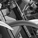
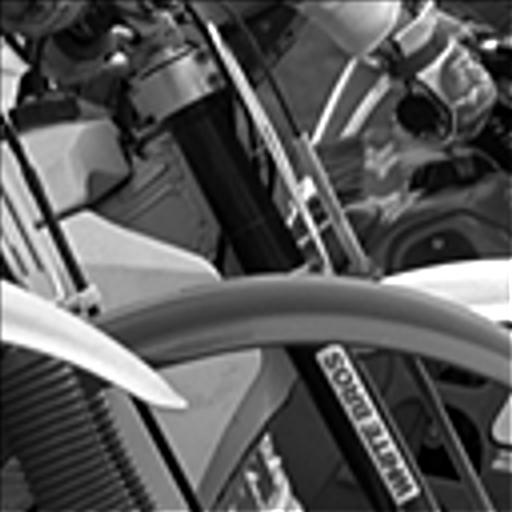
- Fig. 11.7 Results of interpolation the standard Kodak motorcycle image.
- MATLAB script: mdsp_web_changesamp_upsample16_results.m
- Fig. 11.7 (a) Portion of the input image. Output preview: fig11.7a.jpg
- Fig. 11.7 (b) Bilinear interpolator. Output preview: fig11.7b.jpg
- Fig. 11.7 (c) Bicubic interpolator. Output preview: fig11.7c.jpg
- Fig. 11.7 (d) 29 x 29 interpolator obtained with least pth method. image. Output preview: fig11.7d.jpg
- Fig 11.9 Illustration of a downsampling system using the lattices of Example 11.1.
- (a) Selected points of the reciprocal lattices.The Fourier transform of the original signal defined on Gamma is limited to the octagonal region shown, replicated at points of Gamma*.
- MATLAB script: mdsp_web_changesamp_plot_2D_downsample_spect.m
- Output preview: fig11.9a.png
- (b) Output of the downsampling system.
- MATLAB script: mdsp_web_changesamp_plot_2D_downsample_spect_b.m
- Output preview: fig11.9b.png
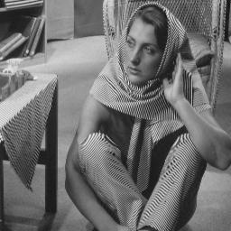
- Fig. 11.10 Downsampling the Barbara image by a factor of two in each dimension. (a) Without prefiltering. (b) With antialiasing prefilter.
- MATLAB script mdsp_web_changesamp_downsample4_barb.m
- (a) Downsampled image without prefiltering. Output preview: fig11.10a.jpg
- (b) Downsampled image with prefiltering. Output preview: fig11.10b.jpg
- (c) Power density spectrum of the input Barbara image. Output preview: fig11.10c.png
- (d) Power density spectrum of the downsampled Barbara image with no prefilter. Output preview: fig11.10d.png
- (e) Power density spectrum of the prefiltered Barbara image. Output preview: fig11.10e.png
- (f) Power density spectrum of the prefiltered and downsampled Barbara image. Output preview: fig11.10f.png
- Design of the antialiasing prefilter (run first). MATLAB script: mdsp_web_changesamp_design_qs_antialiasing_filter.m
- Example 11.3 — Fig. 11.12-11.14 Sampling structure conversion system.
- Fig. 11.12 Input and outout lattices and least dense common superlattice.
- MATLAB script: mdsp_web_changesamp_plot_lattices_example_conversion.m
- Output preview: fig11.12.png
- Fig. 11.13 Frequency domain situation for upconversion from Lambda1 to Lambda3.
- MATLAB script: mdsp_web_changesamp_conversion_examp_spect1.m
- Output preview: fig11.13.png
- Fig.11.14 Frequency domain situation for downconversion from Lambda3 to Lambda1.
- MATLAB script: mdsp_web_changesamp_conversion_examp_spect2.m
- Output preview: fig11.14.png