Chapter 2 Continuous-Domain Signals and Systems
MATLAB code for figures and examples
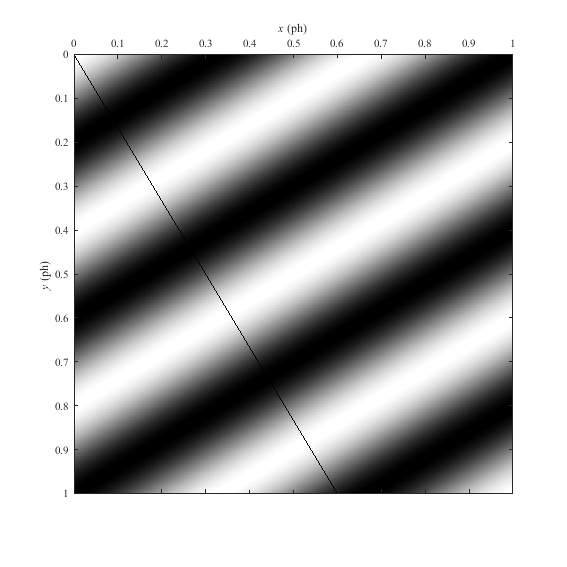
- Fig. 2.4 Sinusoidal signal with u = 1.5 c/ph and v = 2.5 c/ph.
- MATLAB script: mdsp_web_cda_one_sinusoid.m
- Output preview: fig2.4.png
- Fig. 2.5 Zone plate with parameter 1/250 ph.
- MATLAB script: mdsp_web_cda_zone_plate_im.m
- Output preview: fig2.5.png
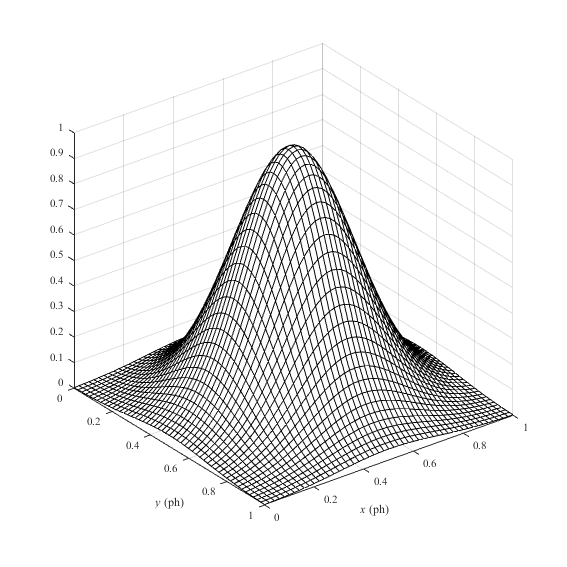
- Fig. 2.6 Visualization of a two-dimensional Gaussian signal with parameter r = 0.2 ph:
- (a) Intensity plot.
- MATLAB script: mdsp_web_cda_gauss_shading.m
- Output preview: fig2.6a.png
- (b) Contour plot:
- MATLAB script: mdsp_web_cda_gauss_con.m
- Output preview: fig2.6b.png
- (c) Perspective plot:
- MATLAB script: mdsp_web_cda_gauss_persp.m
- Output preview: fig2.6c.png
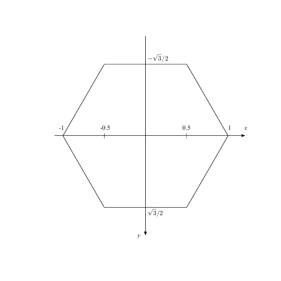
- Fig. 2.12 Regular hexagon with unit side.
- MATLAB script: mdsp_web_cda_unit_hex.m
- Output preview: fig2.12.png
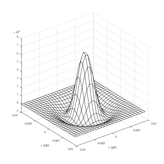
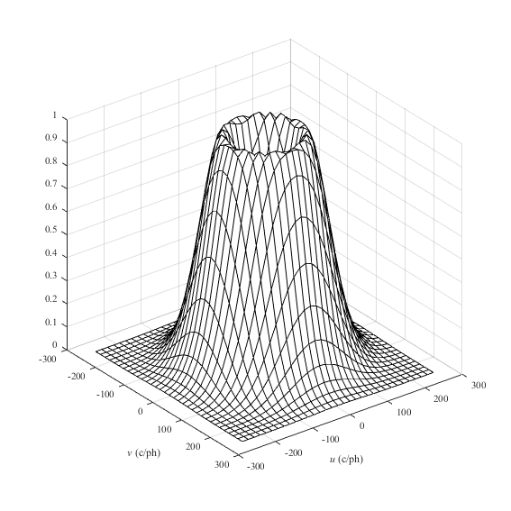
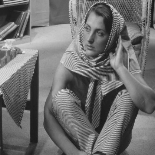
- Fig. 2.13, 2.14 Laplacian of Gaussian filter, impulse response, frequency response and filtered image.
- MATLAB script: mdsp_web_cda_LoG_plots.m
- (a) Negative of impulse response. Output preview: fig2.13a.png
- (b) Magnitude of frequency response. Output preview: fig2.13b.png
- (c) Output of filter applied to Barbara image. Output preview: fig2.14.jpg
- Input Barbara image preview: barb512_gray.jpg