Communication by asynchronous messages - different queuing disciplines

The semantics of FSM modeling

A Finite State Machine (FSM) of Mealy style is a state machine as in UML, where a transition has normally an input and a subsequent output (in addition to the transfer to the next state). Such a transition is like two IOA transition, first an input transition leading to an intermediate state, and then an output transition leading to the next state of the FSM. In the intermediate state, the machine does not accept any other input, it simple prepares for the output transition. In the case of an Extended FSM (as in UML), the transition may also be associated with some update of local variables and the calculation of the effective values of the output parameters.

In the modeling paradigm of Communicating FSMs, the input messages for a given FSM are first placed into an input queue before they are processed by the FSM through the execution of an appropriate transition. There are different queueing disciplines that can be used, such as the following,. Note that we consider a general system architecture which contains many FSMs that communicate with one another.

• Single FIFO queue (also called Common Queue): The messages are placed into the single queue of the machine in the order in which they arrive, and they are processed in FIFO order.
  • One often assumes that there is no transmission delay for the messages (they are placed into the queue of the destination FSM at the time that the source FSM produces the output.
  • This assumption is justified because with interleaving semantics and assuming arbitrary delays, the possible orders in which the messages may be placed into the queue of a given FSM is the same as when all trasnmission delays would be zero.
• Separate queues: Each FSM has a separate queue for each FSM from which it receives messages. In this case the message from each queue will be served in FIFO order, but the machine may decide (based on the existing transitions in its current state, and the messages in the front of each queue) from which queue the next transition should be processed. The message processing order is more flexible than in the single-queue case.
• Saving messages: In certain states, certain messages in the queue may be saved for later processing when the machine is in another state. This feature is included in the SDL language.
• Systematic saving: All messages for which there is no transition in the current state are saved. (Note: This means there is no problem with unspecified receptions).
• Message pool: This means systematic saving without FIFO ordering of message processing, that is, messages in the pool may be processed by the machine whenever it has a corresponding transition from its current state.
  • This approach has some advantages. It is often used for Web Services protocols.
  • It has, however, the problem that some message may remain in the pool without being processed by the receiving FSM. This is a design fault of the system (complementary to the unspecified reception design fault). A well-designed system is stuck-free - a property formally defined in **. Some experimental tools for verifying stuck-freeness have also been developed.

Another semantic variation point (see UML) is the question how unspecified receptions are handled. The following cases are the most popular:

• Avoidance: Unspecified receptions can be avoided by requiring that each FSM is completely specified, that is, it has in each state transitions for all messages in the input alphabet.
  • Note: This leads to overspecification of the system components.
• Design fault: Consider the possibility of the occurrence of an unspecified reception as a design fault which should be avoided by revising the definition of the component behaviors.
  • In an implementation of the FSM model, this may be realized by completing the specification of each FSM by the introduction of a Fail state and transitions for unspecified receptions leading into this Fail state (see Master thesis of Aliaa Alghamdi).
• Ignore the input: An unspecified reception will be ignored by doing a transition back into the current state (without any effect on the local variables).
  • This option is taken in the SDL language.
• Automatic saving: This would be the case for the queueing options Systematic Saving and Message Pool.

In many papers on more theoretical aspects of FSMs, state machines with input queues are described in a formalism that resembles IOA. I will call this approach FSM in IOA notation. With this approach each input-output transition is cut into two transitions, one input and one output. In contrast to the normal FSM semantics, the state after the input transition is a normal state (and not an intermediate state with special properties). This means after an input, another input may be received. Also from a given state, there may be several output transitions - and the machine will have to choose which one to executed (an internal choice). There may also be so-called mixed states from which input and output transitions are possible - this means in this state, the machine may macke a choice between doing an output or processing an input (or if none is present, wait for a while for an input - if none arrives, the basic liveness assumptions requires that finally an output transition must be performed).

The modeling paradigm of FSM in IOA notation is more powerful than the standard FSM modeling paradigm. Therefore the latter is sometimes extended by introducing spontaneous transitions (without input) that may produce output. Such FSM then, may include mixed states as the FSMs in IOA notation.

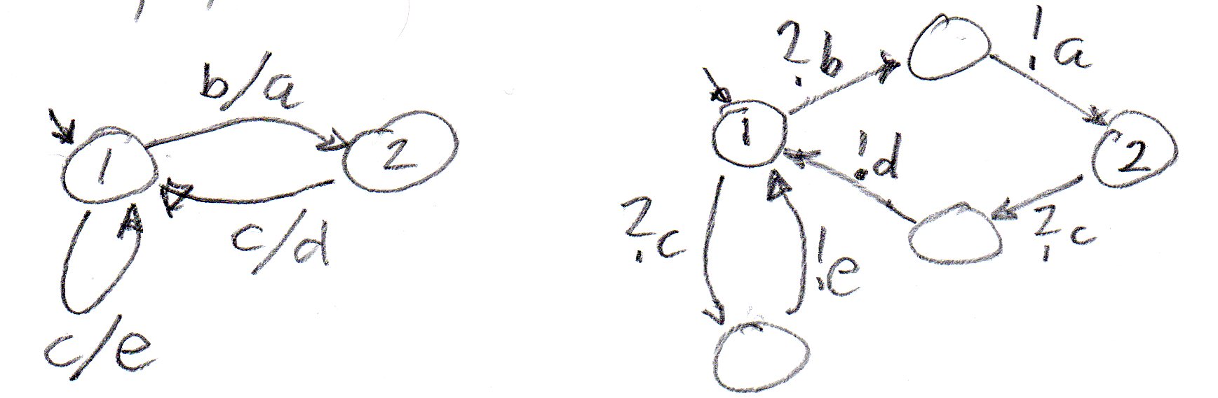
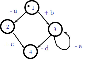
Here are some examples with input alphabet {b, c} and output alphabet {a, d, e} - the notation - means output and + means input. The first two machine have equivlent behavior, that is, admit the same set of traces.

Reachability analysis

The reachability analysis for a system of FSMs is similar as for a system of IOA. The main differences are the following:

• Messages may be in transit (or residing in an input queue before they are processed). This must be taken into account when one defines the global state of the system.
• Message transmission is asynchronous (instead of directly coupled). This means that an input action is coupled with taking a message out of the queue, and an output action is coupled with placing the message into the queue of the destination FSM.

We do not discuss the reachability analysis for all the different semantic variation points that exists for the Communicating FSM model. We describe in the following only the case of two FSM is IOA notation with single FIFO queues. The following text is similar to the definition of reachability analysis given for the IOA modeling paradigm. The changed part of written in blue.

The composition of two FSM models, C1 and C2, with alphabets A1 = I1 union O1, and A2 = I2 union O2, respectively, can be modeled by a global LTS that represents the behavior of these two component FSM and their interactions, in the following called C. The model of C is the following LTS (Note: rules (1) and (2) are the same as for LTS):

1. The states of C are of the form <s1, q21, q12, s2>, where s1 is a state of C1 and s2 is a state of C2, and q12 and q21 are the queues of C2 and C1, respectively.
2. The initial state of C is the set of states <s1-initial, empty, empty, s2-initial> where si-initial are initial states of Ci (i = 1, 2).
3. The transitions of C from a state <s1, q21, q12, s2> are the following:

• reception by C2 for m in O1 and in I2
  • if there a message m at the front of the input queue q21 of C1 and s2 -- ?m --> s2' in C2 : then <s1, q21, q12, s2> -- ?m --> <s1, q21, q12', s2'> (input and output transitions executed jointly; this is output to the environment) where q12 is equal to q12 with the message m removed from the front.
  • if there is a message m at the front of the input queue q21 of C1, but no transition s2 -- ?m --> to any state in C2 : non-specified reception (design error)
  • if there is no transition s1 -- !m --> to any state in C1, but there is the transition s2 -- ?m --> s2' in C2 : no transition in the composition (maybe the transition of C2 will never be executed - this depends on the other states of C1 that may occur jointly with s2)
• sending by C2 of m in I1
  • if there is a transition s2 -- !m --> s2' in C2 : then <s1, q21, q12, s2> --m --> <s1, q21', q12, s2'> where q21' is equal to q21 with the message m appended.
• sending by C2 of m not in I1 (m is sent to the environment)
  • if there is a transition s2 -- !m --> s2' in C2 : then <s1, q21, q12, s2> --!m --> <s1, q21, q12, s2'> where the message m is sent to some FSM in the environment.
• for m in A1 and m not in A2 (C2 is not involved in this interaction - direct interaction between C1 with the environment)
  • if there is a transition s1 -- m --> s1' : then <s1, s2> -- m --> <s1', s2> (transition by C1 alone)
• similarly as above, for C1 and C2 interchanged
• for m in I1 and in I2
  • if there are transitions s1 -- ?m --> s1' in C1 and s2 -- ?m --> s2' in C2 : then <s1, s2> -- ?m --> <s1', s2'> (joint transition when input m comes from environment)
  • if there is a transition s1 -- ?i --> s1' in C1 , but no transition s2 -- ?i --> to any state in C2 : possibly a design error, but this depends on the behavior of the environment (non-specified reception for C2 if input comes from environment when C2 is in this state); otherwise the transition of C1 will never be executed. Similarly, for C1 and C2 interchanged.
• for m in O1 and in O2 : this is not allowed according to what is said above - miss-match of the interfaces between the two components - conflicting output transitions.

Example of reachability analysis

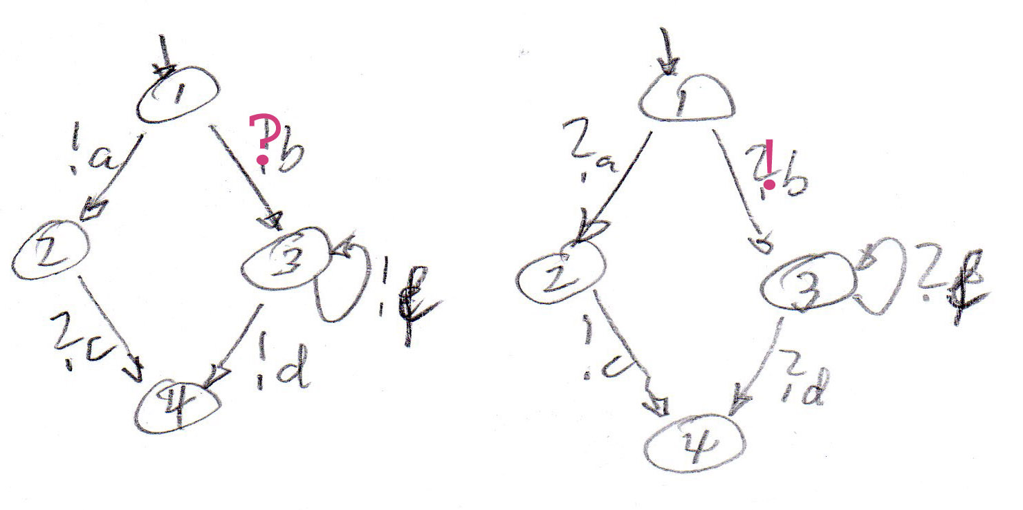
We first consider the third state machine above communicating with its "mirror image", and assuming that IAO communication is used (directly coupled transitions without queuing):

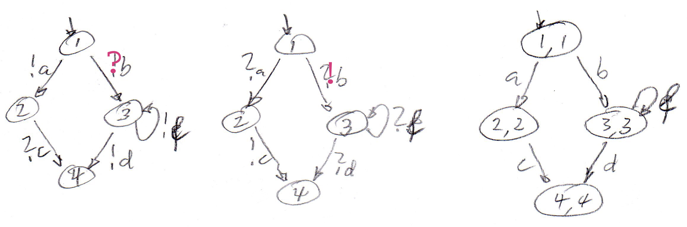
Machine A . . . . . . . . . . . . . . . . . .. . . . Machine B . . . . . . . . . . . . . . . . . . . . The global system

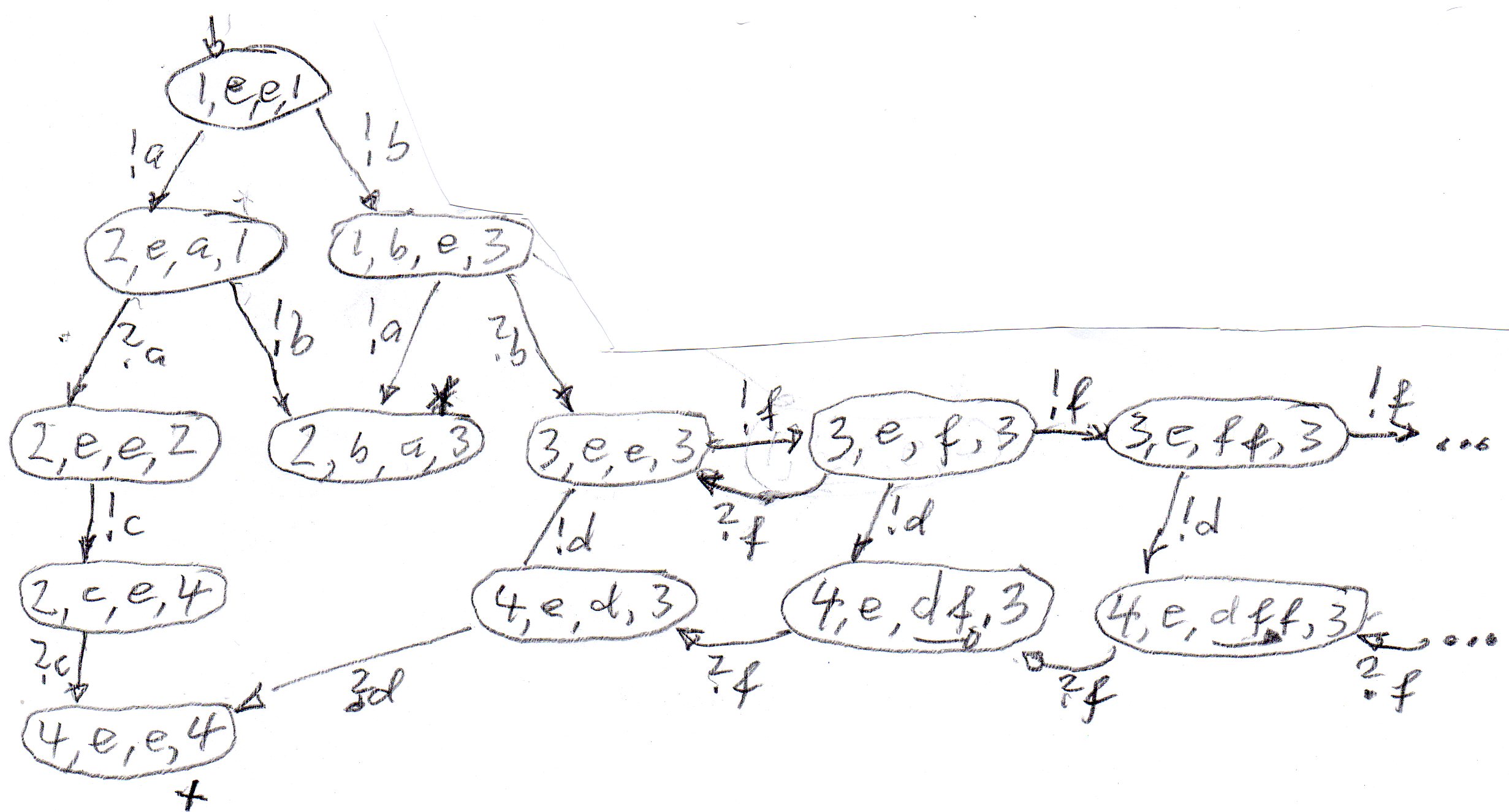
Now we consider that the two machines communicate with message queuing (that is, like FSM in IOA notation). Here is the global reachability grapb (partial, since the queue length of the second machine is not bounded - therefore the number of possible global states is infinite). The notation (s1, q1, q2, s2) means that the first machine is in state s1 and the content of its input queues is q1, and similarly for the second machine. Note that in the global state marked *, there are two unspecified receptions, and the global state marked + is a deadlock - however, this is probably a desired final state, since both communicating machines, are in their respective final state (the only state with no further transitions).

Results of reachability analysis

Reachability analysis allows us to obtain a description of the global behavior of the system that is defined as the composition of several components, each with its specified behavior. For this global behavior, we are interested in two aspects:

• General properties: These are properties that, in general, should be satisfied by any global system behavior. These properties may include the following:
  • Absense of Deadlock (an accessible state without any transition enabled): For a system of communicating FSM, if all queues are empty and no component can produce an output, this is a “global deadlock”; it could be the desired final state. If one of the queues contains an input, but the receiving FSM does not have a transition to consume it, this falls under the category of “unspecified receptions” (see below). One calls “local deadlock” a situation where certain FSMs are blocked forever, but other FSMs continue operations. - Similar for composed LTS.
  • Absense of non-executable transitions: A transition of a given state machine is called “non-executable” if there is no reachable global state in which it could be taken. The system would have the same behavior if this transition was removed from behavior of that component (making it more abstract - more situations of undefined input).
  • Absense of unspecified receptions: If a global state is accessible where one state machine receives a particular input in a state where no transition is specified for that input, this is called unspecified (or non-specified) reception (more detailed discussion). Note: This cannot happen for communicating LTS because they communicate by rendezvous; however, deadlock may occur if one side is not ready to accept the only interaction that the other side can do.
  • Bounded queues: If the size of the queues in all reachable global states is bounded by some integer, then the number of reachable states is finite. The question whether the queues are bounded for a given set of communicating FSMs is in general non-decidable.
  • Self-stabilization: A system of communicating state machines is called “self-stabilizing” if for all (arbitrary) initial states, the system will enter, after some finite time, the normal mode of operation.  (An example is given in [Boch 78]; recent results in this area have been presented by Gouda).
  • Stable states (called “adjoint states” in [Boch 78]): A state vector (representing the states of all component machines) is called “stable” if for each integer L, there is an execution sequence longer than L which leads to a global state corresponding to this vector (with arbitrary content of the queues). It means that, if <s1, s2> is a pair of stable states, then when component 1 is in state s1, the component 2, may be in state s2.
• Specific properties: In our survey paper of 1980 on communcation protocol design, we make the distinction between general properties (see above) and specific properties which depend on the particuar system. Usually, these specific properties are defined by the system requirements. The specific properties represent a more abstract view of the system. When one checks that the analyzed model (the "more detailed model") satisfies the specific properties of the more abstract model, one talks about Model Checking. Note, however, that Model Checking also includes the checking of the general properties above. Note: Some people say that the abstract model is checked to see whether it describes the detailed model; other people say that the detailed model is checked to see whether it satisfies the requirements of the abstract model). Anyway, the abstract model must be defined in some suitable language. Various approaches can be used to describe the abstract model:
  • state machine models (involving only the externally visible interactions) - for instance the service specification for the ABP.
  • assertions associated with the variables and interaction parameters of the analysed model (the "more detailed model")
  • Temporal logic (linear time, or branching time Temporal logic)

Example of system development: See course notes for SEG-2106 , Chapter 3 R - Section: "Sub-systems communicating by message passing"

History of protocol engineering C

The first paper that used state machine modeling of communication protocols was probably the paper describing the Alternating Bit Protocol (ABP) in 1968. My paper of 1978 on Finite State Description of Communication Protocols was the first paper to introduce reachability analysis for verifying that a given protocol and underlying message transmission service provides a given service specification (in this case, reliable data transfer to the sender to the receiver). I used the APB as the main example, but also treated the X.25 protocol which was then the official ITU standard for computer communication over data networks. At the same time, Colin West with colleagues from the IBM Zurich Research Lab had also developed methods for checking that protocol specifications have no deadlock nor unspecified reception, also using reachability analysis based on state machine models (see paper of 1980). They introduced the notion of unspecified reception. All these papers used the modeling paradigm of FSM in IOA notation (see above). During those days, various formalisms were used to describe protocols (see survey of 1980).

An overview of the history of protocol engineering, including the development of the first protocols for computer networks in the 1970ies, is given in my paper Some notes on the history of protocol engineering (or a shortened version with the ABP example). These principles of protocol engineering were applied to a large extend during the standardization development for Open Systems Interworking (OSI) during the 1980ies (see my paper Protocol Specification for OSI from 1990) - however, these protocols were never much used because they were superseded by the wide-spread use of the Internet protocols in the 1990ies.

In the late 1970ies, Colin West, with his colleagues at IBM, developed in interesting reachability analysis tool that helped the protocol designer defining protocols without unspecified receptions (see paper of 1980). Using this tool, the designer could develop the behavior of two (or more) state machines interactively by introducing sending transitions from the different states of the machines. The tool will determine automatically in which state (or states) of the destination machine each output message could be received. These receptions are indicated by the tool, and the designer has to select the state that should be entered after the reception of the message (either a state that already exists, or a new state for the machine in question). Thus, all possible receptions must be handled by the designer and the resulting design will have no unspecified reception. Deadlocks were also detected by the tool - they can be resolved by introducing an output transition in one of the machine states involved in the deadlock - but this is not necessarily a good solution (one may also change the earlier behavior of one of the involved state machines).

Created: October 9, 2014, revised Oct. 2015