Supporting Software Maintenance by Mining Software Update Records

By

Jelber Sayyad Shirabad

Thesis submitted to the Faculty of Graduate and Post-Doctoral Studies in partial fulfillment of the requirements for the degree of

Doctor of Philosophy in Computer Science

Ottawa-Carleton Institute for Computer Science

School of Information Technology and Engineering

University of Ottawa,

Ottawa Ontario Canada

This thesis is also available as a pdf file.

© Jelber Sayyad Shirabad, May 2003

To my father, mother and sister

for their endless love and support

I have yet to see any problem, however complicated, which, when you looked at it in the right way, did not become still more complicated.

Poul Anderson (1926-2001) Science Fiction Writer

Abstract

It is well known that maintenance is the most expensive stage of the software life cycle. Most large real world software systems consist of a very large number of source code files. Important knowledge about different aspects of a software system is embedded in a rich set of implicit relationships among these files. Those relationships are partly reflected in system documentation at its different levels, but more often than not are never made explicit and become part of the expertise of system maintainers. Finding existing relations between source code components is a difficult task, especially in the case of legacy systems.

When a maintenance programmer is looking at a piece of code in a source file, one of the important questions that he or she needs to answer is: ìwhich other files should I know about, i.e. what else might be relevant to this piece of code?î. This is an example of a more general Relevance Relation that maps a set of entities in a software system into a relevance value.

How can we discover and render explicit these relationships without looking over the shoulder of a programmer involved in a maintenance task? We turn to inductive methods that are capable of extracting structural patterns or models from data. They can learn concepts or models from experience observed in the past to predict outcomes of future unseen cases.

This thesis lies at the intersection of two research fields, which has been widely ignored by researchers in the machine learning and software engineering communities. It investigates the application of inductive methods to daily software maintenance at the source code level. Therefore in this thesis we first lay out the general idea of relevance among different entities in a software system. Then using inductive learning methods and a variety of data sources used by maintenance programmers, we extract (i.e. learn) what we call a maintenance relevance relation among files in a large legacy system. In effect we learn from past maintenance experience in the form of problem reports and update records, to be able to make predictions that are useful in future maintenance activities. This relation, which is called the Co-update relation, predicts whether updating one source file may require a change in another file.

To learn the Co-update relation we have performed a large number of experiments using syntactic features such as function calls or variable definitions. We have also performed experiments that use text based features such as source code comments and problem reports, and the combination of these features. The results obtained show that while using syntactic features is encouraging in terms of the predictive power of the results of learning, using text based features yields highly accurate models, with precision and recall measures that make these models viable to be used in a real world setting. As part of the contribution of this thesis we also report on challenges encountered in the process and the lessons learned.

Acknowledgments

I would like to express my deepest gratitude and thanks to my supervisors Dr. Stan Matwin and Dr. Timothy C. Lethbridge for imparting their knowledge and wisdom to me, and their support, care, trust and friendship. I thank Tim for his very generous financial support through the years, which relieved the financial burden associated with my studies to a great extent. I would also like to thank Stan for his support for the last few years which allowed me stay focused on my research at a time that I had to face fluctuations in funds due to external factors. He also generously provided me with a new and more powerful PC in the last year of my study, which speeded up running the experiments quite considerably and was instrumental in allowing me to include some of the more interesting results in this thesis.

Tim was the primary proofreader of my thesis and I would like to thank him for his thorough review of its many drafts. His feedback allowed me to present the thesis and our joint publications in a way that is understandable to an audience who may not necessary have a background in machine learning. I am also grateful to Stan for corrections and comments I received from him especially on machine learning related topics and many pointers he provided me which certainly helped me with improving the quality of my research and this thesis. I have learned a lot from both my supervisors.

I would like to express my appreciation and thanks to the members of my defense committee Dr. Eleni Stroulia the external examiner from the University of Alberta, Dr. Lionel Briand of Carleton University, and Doctors Nathalie Japkowicz and Liam Payton from the University of Ottawa, for their insightful comments and suggestion to improve the quality of this thesis. I am grateful to Dr. Robert Holte for his comments on my thesis proposal and our follow up discussions, which have greatly influenced my research.

Funding for this research was made available by the Consortium for Software Engineering Research (CSER), Mitel Networks, and The Natural Science and Engineering Foundation of Canada (NSERC). The University of Ottawa provided me with an admission scholarship and tuition fee waiver for the first two years of my studies. This was a great help for me and I am very thankful the university for it.

Many thanks to the members of SX 2000 team, the support staff, and the research management at Mitel Networks and in particular Steve Lyon, Steve Szeto, Soo Tung, Ian Duncan, Chris Halford, Peter Perry and Daisy Fung for the assistance they provided.

Special thanks to Dr. Sylvia Boyd who trusted me with teaching Prolog Concepts Laboratory for the first time, and Dr. Lou Birta for his continuous encouragement and friendship.

Over the years I have received excellent software and hardware support from Keith White, Michel Racine, Marc Fortier, Roger Montcalm, and Alan Stewart. Their assistance is greatly appreciated.

My life as a student would have been more challenging if it wasnít for many good people who over years of my study at the University of Ottawa consistently showed their friendship. In no particular order, I would like to thank my colleagues and friends Viviana Nastase, the Azizi family, Francisco Herrera, Gina Gonzalez, Rossana Andrade, Stephane SomÈ, Alan Williams, Masahide Nakamura, Khalid Khidhir, Felipe Contreras, the Yeghikian family, the Zamora family, Nicolas Anquetil, Kathia Oliveira, Amy Yi, Chris Drummond, Artush Abolian, Jack Dadourian, Ana Shannette and Vahik Manookian for their help, caring and many pleasant memories over years. A special thank you goes to Vivi for allowing me to use her computer at the department during those last days before submitting my thesis for the defense. I also thank her for the excellent work she did as my teaching assistant, as I have come to realize the impact a knowledgeable and reliable TA has on the time that I have to spend on teaching a course. Many thanks to my uncle and aunt who are my family in Canada. Visiting them during Christmas and other occasions helped me to unwind and think less about my research. I have enjoyed many of casual conversation we had around the dinner table. At this juncture, let me also thank everyone else who in one way or the other has had a positive impact on my life and study, and who I have omitted in this acknowledgment.

I still remember my motherís expression when I first told her that I was going to Canada to continue my studies. I remember my father, mother, and sisterís face as we said goodbye in the airport. I saw love then, and I have been blessed with their love and unwavering support during all these years that we have been apart. I feel most blessed for having them as my family, and from the bottom of my hart I thank them for their sacrifices and all they have done for me. The road to the PhD had many ups and downs for me. Now that I am at the end of this road, I feel very humbled by the whole experience, but I know my family is very proud of me. As a small token of my appreciation, I am dedicating this thesis to them.

Table of Contents

Abstract ........................................................................................................................ i

Acknowledgments........................................................................................................... iii

Table of Contents........................................................................................................... vii

Index of Figures............................................................................................................... xi

Index of Tables.............................................................................................................. xiii

Chapter 1 Motivation........................................................................................................ 1

1.1 Legacy Software Systems and Software Maintenance.............................................. 1

1.2 Comprehending Legacy Systems............................................................................... 3

1.3 Knowledge Based Software Engineering vs. Application of Inductive Methods in Software Engineering.................................................................................................. 5

1.4 The Goal of the Thesis.............................................................................................. 6

1.5 Definitions and an Application................................................................................. 8

1.6 Contribution of this Thesis..................................................................................... 15

Chapter 2 Related Research.......................................................................................... 17

2.1 Introduction............................................................................................................. 17

2.2 AI and Software Maintenance................................................................................. 18

2.2.1 Knowledge Based Software Engineering........................................................... 19

2.2.2 Knowledge Based Systems Applied to Software Maintenance....................... 22

2.2.2.1 Code Generation (COGEN)...................................................................... 22

2.2.2.2 MACS....................................................................................................... 23

2.2.2.3 Problem Manager (PM)............................................................................. 24

2.2.2.4 Intelligent Program Editor (IPE)................................................................ 26

2.2.2.5 Intelligent Semantic Lisp-program Analyzer (ISLA)................................ 27

2.2.2.6 Maintainers Assistant............................................................................... 27

2.2.2.7 Program Understanding Using Plan Recognition Algorithms.................... 28

2.2.2.8 Model Oriented Reengineering Process for HCI (MORPH)..................... 30

2.2.2.9 Programmerís Apprentice......................................................................... 31

2.2.2.10 Recognizer............................................................................................... 32

2.2.2.11 Program Analysis Tool (PAT)................................................................ 33

2.2.2.12 LASSIE.................................................................................................... 34

2.2.2.13 Knowledge-Based Assistant for Reverse Engineering (KARE).............. 35

2.2.2.14 Summary of Knowledge-Based Maintenance Support Systems............. 37

2.2.3 Inductive Approaches Applied to Software Maintenance............................... 38

2.2.4 Application of Inductive Learning in Software Maintenance........................... 39

2.2.4.1 Fault Density Prediction........................................................................... 39

2.2.4.2 Design Recovery........................................................................................ 40

2.2.4.3 Locating High-Risk Software modules...................................................... 40

2.2.4.4 Software Quality Prediction...................................................................... 42

2.2.4.5 Case-Base Reasoning and Inductive Logic Programming Applied to Software Reuse.......................................................................................... 43

2.2.4.6 Estimating Software Development Effort................................................. 44

2.2.5 Summary........................................................................................................... 45

Chapter 3 Methodology.................................................................................................. 47

3.1. Introduction............................................................................................................ 47

3.2. General Approach.................................................................................................. 49

3.2.1 Pre-Learning Stage............................................................................................ 51

3.2.1.1 Identifying Sources of Data and Knowledge............................................. 51

3.2.1.2 Acquire Data and Knowledge.................................................................... 53

3.2.1.2.1 Creating examples of Relevant and Not Relevant File Pairs............... 54

3.2.1.2.2 Finding Relevant and Not Relevant File Pairs.................................... 54

3.2.1.2.3 Heuristics Based on File Update Information.................................... 56

3.2.1.2.4 Features Used in Defining the Relevance Concept............................. 60

3.2.1.2.5 Features Extracted From the Source Code.......................................... 61

3.2.1.2.6 File Reference Attributes.................................................................... 63

3.2.1.2.7 Data Flow Attributes......................................................................... 65

3.2.1.2.8 Control Flow Attributes..................................................................... 66

3.2.1.2.9 File Name Related Attributes............................................................. 70

3.2.1.2.10 Text Based Attributes...................................................................... 72

3.2.1.3 Preprocessing............................................................................................. 73

3.2.2 Learning Stage................................................................................................... 73

3.2.2.1 Transformation and Encoding.................................................................... 73

3.2.2.2 Learning..................................................................................................... 74

3.2.2.3. Evaluating the Usefulness of the Learned Concept.................................. 75

3.2.2.4. Parameter Tuning...................................................................................... 79

3.2.3 Post Learning Stage........................................................................................... 79

3.3. Limitations of Our Research................................................................................... 80

Chapter 4 Experiments................................................................................................... 81

4.1 Background on the System Under Study................................................................ 81

4.2 Creating Training and Testing Data sets.................................................................. 82

4.3 Removing Class Noise............................................................................................. 82

4.4 Background on Experimental Setup......................................................................... 83

4.4.1 Experiments Using C5.0................................................................................... 84

4.4.2 Experiments With Set Covering Machines....................................................... 95

4.5 The Base Experiments........................................................................................... 101

4.5.1 Creating File Pair Data Sets for the Base Experiments................................... 102

4.5.2 Creating Training and Testing Data Sets for the Base Experiments............... 106

4.5.3 Repeating Relevant Examples......................................................................... 110

4.6 Analysis of the Decision Trees............................................................................. 113

4.7 Using the 1R Algorithm to Create Classifiers....................................................... 114

4.8 Removing Class Noise........................................................................................... 116

4.9 Discretizing Numeric Attributes........................................................................... 119

4.10 Using Text Based Features.................................................................................. 128

4.10.1 Source File Comment Words as Features..................................................... 132

4.10.2 Problem Report Words as Features.............................................................. 135

4.11 Combination of Features..................................................................................... 140

4.11.1 Combination of Syntactic and Source File Comment Word Features.......... 142

4.11.2 Combination of Syntactic and Problem Report Word Features................... 145

4.11.3 Combination of Source File Comment and Problem Report Features.......... 148

4.11.3.1 Juxtaposition of Source File Comment and Problem Report Features.. 148

4.11.3.2 Union of Source File Comment and Problem Report Features............. 151

4.12 Summary.............................................................................................................. 155

Chapter 5 Conclusion and Future Work.................................................................... 159

5.1 Summary and Concluding Remarks....................................................................... 159

5.2 Future Work.......................................................................................................... 165

Appendix A A Three‑Class Learning Problem 169

A.1 Heuristics Based on User Interactions................................................................. 169

A.2 Collecting the Result of Software Engineers Interactions..................................... 170

A.3 Cleaning the Log................................................................................................... 171

A.4 Dividing the Logs into Sessions............................................................................ 171

A.5 Extracting Pairs of Potentially Relevant Software Units...................................... 172

A.6 Example Label Conflict Resolution...................................................................... 173

A.7 Format of log files................................................................................................. 173

Appendix B An Alternative to the Hold Out Method................................................ 177

B.1 Basic Training and Testing File Pairs.................................................................... 178

B.2 Alternatives to Basic Training and Testing File Pairs........................................... 179

B.2.1 Alternative to the Training Set....................................................................... 179

B.3 Precision, Recall and F-Measure Comparisons.................................................... 181

B.4 A Hold Out Evaluation Approach........................................................................ 187

B.5 Summary............................................................................................................... 193

Appendix C Detailed Experiment Results................................................................. 195

Appendix D A Classifier Evaluation Questionnaire................................................ 207

D.1 A Sample Questionnaire....................................................................................... 208

D.2 Instructions Accompanying the Questionnaire.................................................... 211

Appendix E A Sample Decision Tree.......................................................................... 215

E.1 A Decision Tree Learned Form Problem Report Feature Set............................... 215

References .................................................................................................................... 227

Index of Figures

Figure 1.1 Continues and Discrete Versions of a Relevance Relation R......................... 9

Figure 1.2 A System Relevance Graph and its Two System Relevance Subgraphs..... 10

Figure 3.1 Creating a Classifier from a Set of Examples................................................ 48

Figure 3.2 Classifying a New Case................................................................................ 49

Figure 3.3 The Process of Learning a Maintenance Relevance Relation....................... 50

Figure 3.4 The Process of Submitting an Update to Address a Problem Report.......... 53

Figure 3.5 File pairs, Features, and Examples............................................................... 55

Figure 3.6 Relation Between Relevant and Not Relevant Pairs.................................... 60

Figure 3.7 A Decision Tree........................................................................................... 75

Figure 3.8 A Confusion Matrix..................................................................................... 75

Figure 3.9 An ROC Curve............................................................................................. 79

Figure 4.1 ROC Comparison of Stratified Training Experiments................................. 94

Figure 4.2 Creating Training Sets with Different Class Ratios................................... 108

Figure 4.3 ROC Plots of Base Experiments 1 and 2................................................... 109

Figure 4.4 ROC Plots of Base Experiments 3 and 4................................................... 112

Figure 4.5 Comparing the Best ROC Plots when Relevant Pairs are and are not Repeated..................................................................................................... 112

Figure 4.6 ROC Plots of C5.0 and 1R for Base Experiment 3.................................... 115

Figure 4.7 ROC Plots of Class Noise Removal Experiments...................................... 116

Figure 4.8 Decision Tree Size Plots of Class Noise Removal Experiments................ 118

Figure 4.9 ROC Plots for Method 1........................................................................... 120

Figure 4.10 Decision Tree Size Plots of Method 1....................................................... 121

Figure 4.11 ROC Plots for Method 2........................................................................... 123

Figure 4.12 Decision Tree Size Plots of Method 2....................................................... 124

Figure 4.13 ROC Comparison of the Last Stages of Methods 1 and 2......................... 126

Figure 4.14 Decision Tree Size Plots of Methods 1 and 2............................................ 126

Figure 4.15 Creation of Bag of Words Vectors............................................................. 129

Figure 4.16 ROC Comparison of the File Comment and Syntactic Attribute Based Classifiers................................................................................................... 133

Figure 4.17 Creating Source File-Bag of Words Using Problem Reports...................... 135

Figure 4.18 ROC Comparison of the Problem Report and Syntactic Attribute Based Classifiers................................................................................................... 138

Figure 4.19 ROC Comparison of the File Comment Classifiers with and without Syntactic Attributes................................................................................... 143

Figure 4.20 ROC Comparison of the Problem Report Classifiers with and without Syntactic Attributes................................................................................... 146

Figure 4.21 ROC Comparison of the Problem Report Feature Classifiers with Juxtaposed Combination of Used Problem Report and Source File Comment Features Classifiers.................................................................................... 149

Figure 4.22 ROC Comparison of the Problem Report Feature Classifiers with the Union of Used Problem Report and Source File Comment Feature Classifiers.... 152

Figure 4.23 ROC Comparison of the Problem Report Feature Classifiers with the Union of Used Problem Report and Source File Comment Feature Classifiers.... 154

Figure B.1 Effect of Different Test Repositories on the Precision of the Relevant Class Using 1997‑1998 G₂₀ Training Sets 181

Figure B.2 Effect of Different Test Repositories on the Recall of the Relevant Class Using 1997-1998 G₂₀ Training Sets........................................................... 182

Figure B.3 Effect of Different Test Repositories on the F₁ Measure of the Relevant Class Using 1997‑1998 G₂₀ Training Sets 182

Figure B.4 Effect of Different Repositories on the Precision of the Relevant Class Using 1997-1998 NGSL Training Sets....................................................... 184

Figure B.5 Effect of Different Test Repositories on the Recall of the Relevant Class Using 1997-1998 NGSL Training Sets....................................................... 184

Figure B.6 Effect of Different Test Repositories on the F₁ Measure the Relevant Class Using 1997‑1998 NGSL Training Sets 185

Figure B.7 Comparison of the Best Precision Results in Figures B.1 and B.4............ 186

Figure B.8 Comparison of the best Recall Results in Figures B.2 and B.5.................. 186

Figure B.9 Comparison of the Best F₁ Measure Results in Figures B.3 and B.6........ 187

Figure B.10 Comparison of the Best Precision Results in Figure B.7 and 2/3 - 1/3 Split.................................................................................................................... 189

Figure B.11 Comparison of the Best Recall Results in Figure B.8 and 2/3 - 1/3 Split.. 189

Figure B.12 Comparison of the Best F₁ Measure Results in Figure B.9 and 2/3 - 1/3 Split.................................................................................................................... 190

Figure B.13 Comparison of the Best Precision Results in Figure B.7 and 2/3 - 1/3 Repeated Relevant Split............................................................................. 191

Figure B.14 Comparison of the Best Recall Results in Figure B.8 and 2/3 - 1/3 Repeated Relevant Split............................................................................................. 192

Figure B.15 Comparison of the Best F₁ Measure Results in Figure B.9 and 2/3 - 1/3 Repeated Relevant split............................................................................. 192

Figure E.1 Decision Tree Generated by Experiment 16 for Imbalance Ratio 50......... 215

Index of Tables

Table 2.1 Summary of KBSE Systems Discussed....................................................... 37

Table 3.1 Distribution of Files by Their Type............................................................ 58

Table 3.2 Summary of Syntactic Attributes................................................................ 72

Table 4.1 Distribution of SX 2000 Source Code Among Different Files..................... 82

Table 4.2 Training and Testing Class Ratios for Skewed Experiments........................ 85

Table 4.3 Result of Removing Class Noise from Skewed Training Sets...................... 86

Table 4.4 Learning from Less Skewed Training Sets.................................................... 88

Table 4.5 The Effect of Removing Class Noise from Training Sets............................. 88

Table 4.6 Removing Training Relevant Examples from Testing Not Relevant Examples (Noisy Data)................................................................................................ 89

Table 4.7 Removing Training Relevant Examples from Testing Not Relevant Examples (Noise Free Data)......................................................................................... 90

Table 4.8 Training and Testing Class Ratios for Single Combination Experiments..... 90

Table 4.9 Single Combination Versus All Permutation................................................ 91

Table 4.10 Using Relevant Based Approach to Create the Training Not Relevant Examples...................................................................................................... 91

Table 4.11 The Effect of Using Relevant Based Training Files..................................... 92

Table 4.12 Pascal Only Repositories............................................................................. 93

Table 4.13 Results of Experimenting With Pascal Only File Pairs................................ 93

Table 4.14 Training and Testing Repositories Used for Stratified Training Experiments...................................................................................................................... 94

Table 4.15 Conjunction of Balls for Loss Ratio 1 and Distance Metrics L1 and L2..... 98

Table 4.16 Disjunction of Balls for Loss Ratio 1 and Distance Metrics L1 and L2...... 99

Table 4.17 Conjunction of Balls for Loss Ratio 10, Distance Metrics L1, and FSF 1 and 2.................................................................................................................... 99

Table 4.18 Conjunction of Balls for Loss Ratio 10, Distance Metrics L2, and FSF 1 and 2.................................................................................................................. 100

Table 4.19 Disjunction of Balls for Loss ratio 10, Distance Metrics L2, and FSF 1 and 2.................................................................................................................... 100

Table 4.20 Disjunction of Balls for Loss Ratio 10, Distance Metrics L2, and FSF 1 and 2.................................................................................................................. 101

Table 4.21 Data to which File Pair Labeling Heuristics were Applied........................ 102

Table 4.22 Distribution of Group Sizes Created by Co-Update Heuristic................. 104

Table 4.23 Training and Testing Repositories Used in Base Experiments 1 and 2...... 105

Table 4.24 Attributes Used in the Base Experiments.................................................. 107

Table 4.25 Training and Testing Repositories Used in Base Experiments 3 and 4...... 111

Table 4.26 Top Nodes in the Decision Trees of Base Experiment 3........................... 114

Table 4.27 The Normalized Distance of ROC Points from the Perfect Classifier for Class Noise Removal Experiments............................................................. 117

Table 4.28 Decision Tree Size of Class Noise Removal Experiments......................... 118

Table 4.29 The Normalized Distance of ROC Points from the Perfect Classifier for Method 1.................................................................................................... 121

Table 4.30 The Normalized Distance of ROC Points from the Perfect Classifier for Method 2.................................................................................................... 124

Table 4.31 The Normalized Distance of ROC Points from the Perfect Classifier for Methods 1 and 2........................................................................................ 127

Table 4.32 Decision Tree Size Comparison of Methods 1 and 2................................ 127

Table 4.33 The Normalized Distance of ROC Points from the Perfect Classifier for Plots in Figure 4.16.................................................................................... 134

Table 4.34 Decision Tree Size Comparison for Plots in Figure 4.16........................... 134

Table 4.35 The Normalized Distance of ROC Points from the Perfect Classifier for Plots in Figure 4.18.................................................................................... 138

Table 4.36 Decision Tree Size Comparison for Plots in Figure 4.18........................... 140

Table 4.37 The Normalized Distance of ROC Points from the Perfect Classifier for Plots in Figure 4.19.................................................................................... 144

Table 4.38 Decision Tree Size Comparison for Plots in Figure 4.19........................... 144

Table 4.39 The Normalized Distance of ROC Points from the Perfect Classifier for Plots in Figure 4.20.................................................................................... 147

Table 4.40 Decision Tree Size Comparison for Plots in Figure 4.20 and Syntactic Attribute Based Decision Trees................................................................. 147

Table 4.41 The Normalized Distance of ROC Points from the Perfect Classifier for Plots in Figure 4.21.................................................................................... 150

Table 4.42 Decision Tree Size Comparison for Plots in Figure 4.21........................... 150

Table 4.43 The Normalized Distance of ROC Points from the Perfect Classifier for Plots in Figure 4.22.................................................................................... 152

Table 4.44 Decision Tree Size Comparison for Plots in Figure 4.22........................... 153

Table 4.45 The Normalized Distance of ROC Points from the Perfect Classifier for Plots in Figure 4.23.................................................................................... 154

Table 4.46 Decision Tree Size Comparison for Plots in Figure 4.23........................... 155

Table 4.47 Experiments Summary............................................................................... 157

Table 4.47 Experiments Summary (Continued Ö)...................................................... 158

Table A.1 Format of the Log Lines............................................................................. 174

Table A.2 Log Commands and their Meaning............................................................. 174

Table A.2 Log Commands and their Meaning (Continued Ö)................................... 175

Table B.1 Alternatives to Basic Training and Testing Pairs....................................... 180

Table B.2 Alternatives to Basic Training and Testing Pairs (Extended Version)....... 188

Table B.3 Training and Testing Sets Using the Hold Out Method with Repeated Relevant Examples..................................................................................... 191

Table C.1 Detailed Data for Base Experiment 1 (Table 4.24 First Half).................... 196

Table C.2 Detailed Data for Base Experiment 2 (Table 4.24 Second Half)................ 196

Table C.3 Detailed Data for Base Experiment 3 (Table 4.26 First Half).................... 197

Table C.4 Detailed Data for Base Experiment 4 (Table 4.26 Second Half)................ 197

Table C.5 Detailed Data for Experiment 5.................................................................. 198

Table C.6 Detailed Data for Experiment 6 (Single Copy Noise Removal)................. 198

Table C.7 Detailed Data for Experiment 6 (Multi-Copy Noise Removal)................. 199

Table C.8 Detailed Data for Experiment 8.................................................................. 199

Table C.9 Detailed Data for Experiment 9.................................................................. 200

Table C.10 Detailed Data for Experiment 11................................................................ 200

Table C.11 Detailed Data for Experiment 12................................................................ 201

Table C.12 Detailed Data for Experiment 13................................................................ 201

Table C.13 Detailed Data for Experiment 14................................................................ 202

Table C.14 Detailed Data for Experiment 15................................................................ 202

Table C.15 Detailed Data for Experiment 16................................................................ 203

Table C.16 Detailed Data for Experiment 17................................................................ 203

Table C.17 Detailed Data for Experiment 18................................................................ 204

Table C.18 Detailed Data for Experiment 19................................................................ 204

Table C.19 Detailed Data for Experiment 20................................................................ 205

Table C.20 Detailed Data for Experiment 21................................................................ 205

Chapter 1

Motivation

This thesis is devoted to the development and testing of an approach to extract models of a software system that are geared towards assisting software maintainers. The objective here is to learn relations from the past maintenance experience that could be useful in future source code level maintenance activities.

1.1 Legacy Software Systems and Software Maintenance

Legacy software systems are a fact of life in the software engineering community. Many important software systems controlling essential aspects of modern society were developed many years ago. Legacy systems are old systems that still need to be maintained [Sommerville 2001 pp. 582]. It was estimated that in 1990 there were 120 billion lines of code in existence, and at the time the majority of those systems were already considered to be legacy systems [Ulrich 1990][1].

Most legacy systems exhibit the following properties:

… They are old

… They are large

… They are essential for the operation of the organization which uses them

… The existing documentation about them is often incomplete or out of date

… Many of them were designed before the time of structured programming [Choi and Scacchi 1990]

… They have been developed and modified by several people over many years

… There is no single person who possesses a complete understanding of the system

Although systems written in the 1960ís and running on mainframe systems are classical cases of legacy systems, in practice much newer systems developed in the 1980ís and 1990ís, using structured design and other modern techniques are also considered to be legacy at the beginning of the twenty-first century.

According to ANSI/IEEE standard 729-1983, maintenance is the ìmodification of a software product after delivery to correct faults, to improve performance or other attributes, or to adapt the product to a changed environmentî [Chikofsky and Cross 1990 p. 14].

It is known that software maintenance is a time consuming and costly part of the software life cycle. Whether newer software development technologies, such as object orientation, have been effective in practice to alleviate the maintenance burden, is perhaps debatable, but the above statement has been, and is, true for legacy software systems.

While design decisions and the rationale for them are sometimes documented, more often modifications to the source code are the main or the only indication of design changes [Rugaber et al 1990 p. 46]. The lack of up to date requirement, design and code documents has played a major role in making maintenance a difficult, expensive and error prone task.

The cost of maintenance varies widely depending on the application domain. It can range from broadly comparable with system development cost, to up to four times as high as the cost of development for real time embedded systems[2].[Sommerville 2001 p. 607]. There have also been reports of extreme cases in which maintenance cost has been as high as 130 times the development cost [Boehm 1975]. Other researchers have suggested that on average 67% of the total cost of the product can be attributed to maintenance [Lientz, Swanson, and Tompkins 1978][Schach 2002 p. 494]. While [Tracz 1988] put this number close to 70% [Tracz 1988], there are others who suggest an 80-20 rule, which says 20% of the development work is performed during original application development, and the other 80% is performed during maintenance [Conger 1994 p. 740], and the indications are that the cost is likely to increase [McCartney 1991 p. xvii]. [Shari 2001 p. 479] suggests that this increase in the cost of maintenance in the first decade of the new century to be 80% of a typical systemís lifetime cost.

Software maintenance has been referred to as a severe problem [McCartney 1991 p. xviii], or even as being the most difficult of all aspects of software production [Devanbu and Ballard 1991 p. 26] [Schach 2002 p. 494].

Yet despite developing a general understanding of the importance of maintenance in the software life cycle, and an abundance of very large legacy software, academia has not paid as much attention to the topic as it deserves. The papers related to software maintenance are less than 1% of the papers annually published on software topics [Kwon et al 1998 p.1].

1.2 Comprehending Legacy Systems

Four kinds of maintenance activities are:

… Corrective which is concerned with fixing reported errors

… Adaptive which means changing software to accommodate changes in the environment such as new hardware

… Perfective which involves implementing new requirements (enhancement) [Sommerville 2001 p. 605]

… Preventive, also known as software reengineering, which makes changes to computer programs so that they can be more easily corrected, adapted, and enhanced [Pressman 2001 p. 23].

About 20 percent of maintenance work is dedicated to ìfixing mistakesî. The remaining 80 percent is dedicated to adapting the system to a new external environment, implementing enhancement requests from users, and reengineering an application for future use [Pressman 2001 p. 805].

Regardless of the type of maintenance, to maintain a software system one needs to understand it. Better understanding of the software system will assist the maintenance programmer in performing his or her task.

One of most important research areas related to software maintenance is Reverse Engineering. Reverse Engineering is the process of analyzing a system to:

… Identify its components and the relations among them;

… Create an alternative representation for the system at the same or higher level of abstraction

Two widely discussed areas of reverse engineering are redocumentation and design recovery.

Redocumentation involves providing alternative views of a system at relatively the same abstraction level. For example data flow, or control flow diagrams of a system.

Design recovery uses domain knowledge, external information, and deductive and fuzzy reasoning to identify higher level abstractions than the ones that can be obtained by examining the system directly [Chikofsky and Cross 1990 p.15].

In general, most tools developed to assist programmers with comprehending software start from the source code and try to present it in a more abstract level that is easier for a human to understand.

Traditional reverse engineering tools supporting redocumentation mostly rely on static source code analysis methods [Palthepu et al 1997]. They provide graphical views of the interconnections between components of the software system, sometime at different levels of abstraction, but tend to leave the answer to the question of the relation of components to each other in the context of software maintenance to the software engineer. Examples of systems that provide such a capability are Rigi, Imagix4D, and SNiFF++ [Bellay and Gall 1996]. The software engineer should make this decision by browsing through provided information. This becomes more problematic, when the relation is non-trivial and is influenced by a combination of other relations among components.

According to Biggerstaff, ìDesign recovery recreates design abstractions from a combination of code, existing design documentation (if available), personal experience, and general knowledge about problem and application domain. In short, design recovery must reproduce all of the information required for a person to fully understand what a program does, how it does it, why it does it, and so forth. Thus, design recovery deals with a far wider range of information than found in conventional software engineering representations or codeî [Biggerstaff 1989 p. 36].

In relatively recent years there has been a revival of emphasis on the importance of knowledge and its incorporation in reverse engineering tools [Clayton et al 1998 p. 76][Bellay and Gall 1998][Kontogiannis 1995 p. 95]. Such systems in effect will fall into the intersection of Reverse Engineering and Knowledge Based Software Engineering (KBSE).

1.3 Knowledge Based Software Engineering vs. Application of Inductive Methods in Software Engineering

The application of artificial intelligence technology to software engineering is known as Knowledge Based Software Engineering (KBSE) [Lowry and Duran 1989 p.243]. While this definition is fairly broad, most KBSE systems explicitly encode the knowledge that they employ [McCartney 1991 p. xix]. KBSE systems designed for assisting software engineers in low-level everyday maintenance tasks have the potential of representing and deducing the relations among components of a software system at the expense of requiring a fairly extensive body of knowledge and employing, sometimes computationally demanding, deductions and other algorithms. In other words most such systems are fairly knowledge rich. As we will discuss in Chapter 2, KBSE systems tend to employ expert systems or knowledge bases as their underlying technology.

While there has been a fair body of work that has applied deductive methods to different aspects of software engineering, the application of inductive methods (also known as Machine Learning) in software engineering has received far less attention. In Chapter 2 we will review some of the research conducted in this area.

It has been argued that learning systems have the potential of going beyond performance of an expert so as to find new relations among concepts by examining examples of successfully solved cases. In effect this could allow the incorporation of knowledge into a system without the need for a knowledge engineer. In other words, using inductive methods to extract the knowledge that helps a software engineer in understanding a software system, is an alternative to more traditional KBSE techniques. We should point out that this does not mean that one cannot incorporate expert knowledge in the process. On the contrary it is believed that such a contribution can increase the potential gain obtained by using inductive methods [Weiss and Kulikowski 1991 p. 3]. However, as it will become clearer in Chapters 2 and 3, unlike KBSE systems, expert knowledge is not coded in the form of a large knowledge base.

1.4 The Goal of the Thesis

Software engineers who maintain legacy software systems usually work very close to the source code. This often implies that they have to know about the components of the system involved in a problem e.g. files, routines, and the interconnection of these components with other components of the system. As will be discussed in Chapter 2, KBSE research, in general, has been concerned with topics that may not be directly addressing software maintenance activities, or at least not at this level of granularity. Although we will present examples that provide assistance at the source code level, most of them are prototypes that are not applied to real world software systems. This general trend of lack of focus on software maintenance is partly due to the ideal of KBSE that, if fully implemented, will remove the source level maintenance activities by automating the process of generating the software from its specification. While this would be of great value for systems to be created in the future, it does not apply to the large body of currently existing legacy systems.

On the other hand, inductive methods, which have been successfully used in different domains, have not been extensively applied to software maintenance. Software maintenance requires knowledge and experience. Maintenance assistant tools can benefit from such knowledge. Inductive methods are capable of extracting structural patterns or models from data. They can learn concepts from experience observed in the past to predict outcomes of future unseen cases. These methods do not require a knowledge acquisition step necessary to build a knowledge based system. Consequently, there seems to be a great opportunity in using these methods to aid software engineers in software maintenance

Broadly speaking, the aim of this thesis is to investigate the application of inductive methods, which are the focus of the field of Machine Learning [Mitchell 1997], to source code level daily software maintenance. This is the intersection of two research fields, which has been widely ignored by researchers in these communities. Considering the importance of maintenance, and the maturity of inductive learning methods, we believe the time has come for the software engineering and machine learning researchers to join forces in assisting software engineers in maintenance of software systems, especially legacy software at the source code level. We also believe research in this area can benefit machine learning community by providing a rich and nontrivial application area that challenges the community to improve their existing techniques, algorithms, and the overall current state of the technology.

Using inductive learning methods and a variety of data sources used by maintenance programmers, we extract, or learn, what we call a maintenance relevance relation among entities in the system under consideration. This can be seen as a design recovery process. The hope is that the extracted relation will inform and assist the maintenance programmer to understand some of existing complex relations or interactions within the target system. These relations may reveal the intrinsic interconnections between different component of the subject system which:

… may or may not be documented;

… are the consequent of the original design and implementation decisions, or side effects of changes that the system has gone through over its life time

Therefore in this thesis we lay out the general idea of relevance among entities in a software system, and then proceed to apply inductive learning methods to learn a specific relation which is geared towards the daily maintenance task. As part of the contribution of this thesis we report on challenges encountered in the process, the lessons learned, and the results that are achieved, whether positive or negative. Since research in the intersection of machine learning and software engineering is very rare, we strongly believe in the value of reporting negative results as it may help researchers in adjusting their expectations and avoiding pitfalls.

1.5 Definitions and an Application

In this section we provide the definitions of Relevance Relation and other concepts closely related to it. We will also describe a specific application that aims to extract a useful relevance relation in the context of software maintenance.

Definition: A Software Entity is any semantically or syntactically valid construct in a software system that can be seen as a unit with a well defined purpose[3].

Examples of software entities include documents, source files, routines, modules, variables etc.

Definition: A Predictor is a relation that maps one or more software entities to a value reflecting a prediction made about these entities.

Definition: A Relevance Relation is a predictor that maps two or more software entities to a value r quantifying how relevant i.e. connected or related, the entities are to each other. In other words r shows the strength of relevance among the entities. Therefore, ìrelevantî here is embedded in, and dependent on, the definition of the relation.

In its most general form, a relevance relation maps the entities into a real number between 0 and 1 showing the strength of the relevance among them. In this setting 0 stands for the lack of relevance, and 1 shows 100% relevance. We call such a relation a Continuous Relevance Relation. However, a real number may not necessarily always be the best choice, in which case the strength may be one of k discrete values. In the later case we call R a Discrete Relevance Relation. For instance if k is two, we could have a Boolean relevance relation R that maps entities e₁,Ö, e_n (n„2) to true if, based on the definition of R, the entities e₁,Ö, e_n are Relevant to each other. If R maps e₁,Ö, e_n to a false value, this means that, based on the definition of R, e₁,Ö, e_n are Not Relevant to each other.

Figure 1.1 shows the two varieties of relevance relations.

Figure 1.1 Continues and Discrete Versions of a Relevance Relation R

Definition: A System Relevance Graph for R or SRG_R is a hypergraph where the set of vertices is a subset of the set of software entities in the system. Each hyperedge in the graph connects vertices that are relevant to each other according to a relevance relation R[4]. A System Relevance Subgraph SRG_R,r is a subgraph of SRG_R where software entities on each hyperedge are mapped to a relevance value r by relevance relation R.

Figure 1.2-a shows a system relevance graph for a system with five entities e₁,Ö, e₅ and a relevance relation R that maps every two entities to one of two relevance values e.g. a Boolean relevance relation. Figures 1.2-b and 1.2-c show the subgraphs formed for each of these relevance values. Assume the solid lines correspond to a mapping to a true value and the broken lines correspond to a mapping to false value. In this case, the above graphs show that based on the definition of relation R the following pairs of entities are relevant to each other,

(e₁,e₃), (e₁,e₅), (e₃,e₅), (e₄,e₅)

and the following pairs are not relevant to each other,

(e₁,e₂), (e₁,e₄), (e₂,e₃), (e₂,e₄), ,(e₂,e₅), (e₃,e₄)

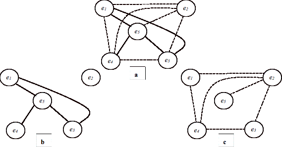
Figure 1.2 A System Relevance Graph and its Two System Relevance Subgraphs

If SRG_R has n vertices, and relevance relation R maps m entities to a relevance value, the maximum number of system relevance subgraphs is:

number of hyperedges with m vertices in a graph with n vertices

Definition: A System Static Relevance Graph or SSRG_R is an SRG in which R is defined in terms of static relations[5] in the source code e.g. calls or called‑by relations for routines.

The number of nodes in an SRG in a given release of a software system is constant. Therefore the topology of the SRG only depends on the definition of the relevance relation among the nodes. This means that a software system can be depicted by different SRGs. Two SRGs of the same system may share one or more connected sub-graphs suggesting the possibility of the existence of a meta‑relation between two relevance relations. For example an SRG based on the Is-In-Subsystem Relevance Relation and an SRG based on the Documents-Entity Relevance Relation may share a common sub‑graph suggesting that there is documentation for a subsystem.

We provided the definition of redocumentation and design recovery in section 1.2. Note that SRGs can be used in both cases during a reverse engineering effort. The level of abstraction represented by an SRG depends upon the definition of the relevance relation it is based on. The notion of relevance relation as defined in this thesis is flexible, in that the definition of the relation can capture simple or very complex interactions between the entities mapped by the relation. The definition can be based on a combination of the existing relations among the entities themselves, or between the entities and other entities in the system. For instance a relevance relation between files can be defined in terms of the file inclusion relation among files, and a variable reference relation among files and variables to which they refer.

Most organizations that produce software have access to tools that allow programmers to browse or query low level static source code relations, such as ëwhat are the routines calledí or ëwhat are the variables referred to in a fileí. TkSee [Lethbridge and Anquetil 1997][Lethbridge 2000], a tool in use at Mitel Networks[6] to browse and explore software systems, is an example of this. By using such tools and studying source code it is possible to reverse engineer and associate design decisions with the source code, however some SSRGs can speed up this process considerably. TkSee uses a database that stores information generated by parsing the source files in the system. For instance, for each routine r in the software system, this database keeps a list of routines called by r[7]. Using this information one can create an SSRG_{calls(ri,rj)ÆBoolean} in which calls is a relevance relation that maps two routine entities r_i and r_j to true if r_i calls r_i in the source code, and false otherwise. Note that SSRG_{calls(ri,rj)ÆBoolean} is an example of an SRG that can be used in redocumenting a system.

However, SRGs that are based on relevance relations defined in terms of a single source code level relation form the most basic and least complex subset of all possible SRGs. Although these SRGs can be extremely useful for a developer in the maintenance task, they fail to capture non trivial relations that exists among entities in a software system.

In this thesis we investigate the existence of other relevance relations that may assist a maintenance programmer in his or her job. To be more specific, within the context of maintenance activity, we are trying to seek the answers to the following questions:

… Using a combination of static source code relations and/or other sources of information, can we find other useful and non trivial relevance relation(s) in a software system?

A Static Relevance Relation R is defined in terms of static source code relations.

Within the context of the system under study, and among different static relations in the source code that are candidates to be used in the definition of R, we would like to investigate the existence of an importance order among these relations. In other words, we would like to be able to answer the following question:

What are the more important static relations which a maintenance programmer should be aware of [8]?

We believe finding a Maintenance Relevance Relation (MRR) could provide an answer to these questions. Such a relation should somehow incorporate information about the changes applied to the system as part of the maintenance process. Consequently, it has the potential to reflect the interconnections among the entities of a system, which are influenced by the changes applied to the system. Such interconnections may or may not conform to the original or perceived design of the system. Instead they could show the existence and interplay of the actual interconnections among the entities, which cause changes in one entity to influence another ones

The definition of software entity given above is very broad in nature. It ranges from a single variable, to the whole system. In the context of software maintenance activity, there is a much smaller set of software entities that seem to be interesting. Examples of such software entities are files, routines, variables, modules, subsystems and documents.

When a maintenance programmer is looking at a piece of code, such as a file or a routine, one of the important questions that he needs to answer is:

ìwhich other files should I know about, i.e. what else might be relevant to this piece of code ?î.

While this is a question faced in daily source level maintenance tasks, the ability to answer it is essential in understanding and maintaining any software system regardless of the type of maintenance activity.

In this thesis we will be focusing on a special kind of SRG in which the nodes are files[9]. We would like to learn a special class of maintenance relevance relations called the Co‑update relation:

Co-update(f_i, f_j) Æ {Relevant, Not-Relevant} where,

i ¼ j and f_I and f_j are any two files in the system.

Co-update(f_i, f_j) Æ Relevant means that a change in f_i may result in a change in f_j, and vice versa[10].

A relevance relation such as Co-update could be used to assist a maintenance programmer in answering the above question about files.

To learn the Co-update MRR we propose the application of inductive learning methods to the data extracted from[11] the following sources of data corresponding to a real word legacy system[12]:

… Static source code analysis

… Historical maintenance records

In other words we mine[13] these sources of data to extract the Co-update relation. The idea here is that such a relation learned from the examples of the past maintenance experience could be used to assist the software engineers, specially the newcomers to the team, in future similar maintenance activities.

In theory there is no need to restrict the number of entities to be two. Our decision to learn this special case of relevance relation is based on the following observations:

… A two-entity relation provides the most basic kind of relevance relation in terms of number of entities. This also implies that it can potentially capture more general interconnections among entities of the system. A relation with three or more entities is more restricted than the basic two‑entity relation; since, by its nature, it is a more constrained and specialized form of relation.

… On a more pragmatic note, as one would expect there are usually fewer examples of individual changes involving larger numbers of entities. As will be discussed in Chapter 4, this is also the case for the particular software system used in this study.

It could also be argued that a mapping to a value between 0 and 1 is a better choice. Our more restricted definition is partly due to the learning method that we have experimented with, namely decision tree learning, and partly due to the fact that in a large software system SRG can be very complex. It is not clear to us whether providing a software engineer with a large set of objects with different relevance rankings will be more beneficial than providing him or her with a smaller set that is believed to contain the relevant objects. Of course a real valued variable can be easily discretized to a Boolean variable, however this will introduce the issue of finding the proper threshold value[14].

One of the challenges that we have faced in our research is labeling the examples from which the above MRR is learned. As will be discussed in Chapter 3, this thesis also proposes heuristics to automatically label the examples, without direct involvement of expert software engineers.

The remainder of this thesis is structured as follows:

In Chapter 2 we present a subset of research conducted in the area of software maintenance that is relevant to the subject of this thesis. We will cover research in KBSE and the application of inductive methods to software maintenance. Chapter 3 will provide the details of the method used to learn a Maintenance Relevance Relation. In Chapter 4, we present the experiments we have performed and results we have obtained. Chapter 5 will discuss our conclusions and plans for future work.

1.6 Contribution of this Thesis

Below we list the contributions of this thesis, i.e. the specific technical issues that to the best of our knowledge were not addressed before, and whose solutions presented in this work add to the state of the art in either machine learning or software maintenance methods:

… Proposing a representation of the maintenance task conducive to the use of machine learning.

… Engineering attributes such that on the one hand they can represent properties of software modules and on the other hand, values for these attributes can be acquired from the source code and software maintenance records.

… Producing a large repository of examples[15] from real-life data appropriate for the use of machine learning tools and techniques.

… Experimenting with a number of machine learning methods including decision tree learning, one rule learner, and set covering machines to learn the Co-update maintenance relevance relation and running empirical comparisons of these methods.

… Setting up an experimental protocol for the above including performing more than 570 training and testing runs using the syntactic attribute set, collecting the results, representing them in the form of ROC curves, tables etc.

… Analyzing the results and drawing conclusions about the relative performance of different training/testing split methods, learning methods, and example refinement techniques such as class noise removal etc.

… Introducing the textual attributes which exploit the semantic information implicit in the source file comments and problem reports

… Performing more than 140 experiments with textual attributes and their combinations together and with syntactic attributes. Collecting results and representing them in the form of variety of tables and plots including ROC curves

… Analyzing the results and drawing conclusions about on the relative performance of source file comment, problem report, and combination feature sets

… Preparing and submitting (at the time of this writing) several research publications. Publishing of [Sayyad Shirabad et al 2000, 2001]

Chapter 2

Related Research

2.1 Introduction

It is a known fact that software maintenance is a time consuming and costly part of software life cycle.

Software maintenance encompasses a wide range of topics including reverse engineering, re-engineering, program transformation, program comprehension, impact analysis, regression testing, reuse, software configuration management, web‑based software maintenance, maintenance process models, and maintenance standards [Kwon et al 1998 p.3].

Considering the wide range of topics falling under the umbrella of software maintenance, no single method or paradigm is expected to provide an answer all of its problems. Our focus is assisting maintenance programmers with the following problem:

When a maintenance programmer is looking at a piece of code, such as a source file, one of the important questions he needs to answer is,

ìWhich other files should I know about, i.e. what else might be relevant to this piece of code ?î.

As discussed in Chapter 1, to provide an answer to this question we will learn a special kind of relevance relation among files in the system called the Co-update Maintenance Relevance Relation. We do this by applying machine learning techniques to data sets created by extracting information from the source code and program update history

The more traditional approach to the application of AI to software engineering has focused on the usage of expert systems and more generally, knowledge based techniques. However, the lack of direct attention to support maintenance programmers can also be seen in KBSE community research. In the relatively recent ICSE 16 workshop on Research Issues in the Intersection between Software Engineering and Artificial Intelligence, the discussions were about Knowledge representation and acquisition, reuse and reverse engineering, validation and verification, and software process [Kontogiannis and Selfridge 1995 p. 94]. However maintenance was identified as being one of the areas of high cost leverage [Kontogiannis and Selfridge 1995 p.96].

In the following section we will review the research projects that employ AI technology, and which we believe are directly applicable to the daily task of software maintenance. In general, these projects fall in one or more of reverse engineering, re-engineering, program transformation, and program comprehension research areas.

2.2 AI and Software Maintenance

Artificial intelligence is one of the oldest research areas in computer science. The Dartmouth Summer Research Project on Artificial Intelligence, organized in 1956 by John McCarthy, has been considered by many the birthplace of AI [Russell and Norvig 1995]. To that extent, AI covers a large body of methods and algorithms. Software engineering has been an application target for AI since the early 1980ís, when research in Knowledge Based Software Engineering (KBSE) started[16]. In general, the methods used in traditional KBSE rely heavily on coded knowledge and sometimes deductive methods. On the other hand, inductive classification methods that are mostly considered to be part of Machine Learning research, attempt to extract models of the subject of interest from a set of labeled examples, without encoding a large amount of knowledge.

In following two sections, we will survey some of previous research that could be considered relevant to this thesis topic. Section 2.2.1 focuses on KBSE, while section 2.2.2 presents research that employs inductive methods.

2.2.1 Knowledge Based Software Engineering

In 1983, the Rome Air Development Center (now Rome Laboratory) published a report calling for the development of a Knowledge-Based Software Engineering Assistant (KBSA) which would employ artificial intelligence techniques to support all phases of the software development process [Green et al 1983]. This initiative eventually evolved into KBSA conferences, which later were renamed as Knowledge-Based Software Engineering (KBSE) conferences, and as of 1996 as Automated Software Engineering Conferences.

Knowledge Based Software Engineering, KBSE, is the application of AI technology to software engineering [Lowry and Duran 1989 p.243]. Expressed another way, it is an approach that integrates methods from AI and software engineering [McCartney 1991 p. xvii]. The prevalent feature of KBSE technology, as far as AI is concerned, is the use of knowledge-based technology through explicit coding of the knowledge. Practically, the focus of AI is dealing with knowledge in terms of representation, reasoning, and extracting useful information from large amounts of it [McCartney 1991 p. xix].

While different people have used the term ìknowledge baseî to refer to different things, it seems that the following two definitions are widely applicable across different projects

A knowledge base is:

… ìA collection of simple facts and general rules representing some universe of discourseî [Frost 1986 p. 3], or

… ìA database augmented with the rules for reasoning about the data and inference engine that applies the rulesî [Lowry and Duran 1989 p. 245]

An alternative definition that includes the notion of inheritance and type is:

… ìA knowledge base is a collection of interrelated concepts[17]î [Lethbridge T.C. 1994 pp. 193, 190].

To go beyond capabilities of CASE tools of the 1980ís, KBSE uses knowledge-based and other AI techniques. The overall objective is to provide intelligent computer based assistance for all parts of the software life cycle [Lowry and Duran 1989 p. 245].

According to Green, KBSE has the following five goals: [Green et al 1983 pp. 381-382]

… ìTo formalize the artifacts of software development and software engineering activities that produce these artifacts [Scherlis and Scott 1983].

… To use knowledge representation technology to record, organize, and retrieve the knowledge behind the design decisions that result in a software system.

… To produce knowledge-based assistance to synthesize and validate source code from formal specification. This will enable maintenance to be performed by altering the specification and then replaying the steps for synthesizing source code, with appropriate modifications. There is also a need for knowledge-based assistance to recover high level specifications from source code.

… To produce knowledge-based assistance to develop and validate specifications.

… To produce knowledge-based assistance to manage large software projects. [Lowry and Duran 1989 pp. 245-246].î

The third goal above sheds some light on why maintenance, particularly at the source code level, has not been the primary focus of the KBSE research community. According to Lowry, the view of KBSE regarding the software evolution and maintenance envisions the changes happening by modifying the specification and re-deriving implementation rather than by directly modifying the implementation. This is a fundamental change in approach to the software life cycle [Lowry and Duran 1989 p. 245].

From early days of KBSE, researchers have attempted to create systems that will allow the synthesis of programs by going from a formal specification to executable code. Some of the approaches to the problem are theorem proving, transformational implementation, and interactive programming environments. [McCartney 1991 p. xxi].

The above view is perhaps very attractive for forward engineering. Once the technology is feasible and software is created in this manner, it could also be maintained by altering the specification and regenerating an updated version of the system. Some of the issues with this point of view of software development/maintenance:

… The researchers have mostly focused on the application of purely deductive methods in theorem proving which have the following problems:

… The proof procedures are computationally expensive, which means that large programs can not be produced

… These techniques require that the user provide a formal domain theory and specification, which is expensive and demands skills which are not commonly possessed by the average programmer. [McCartney 1991 p. xxii].

… There exist a large number of legacy software systems that have not been specified formally. It is highly unlikely that these systems will ever be formally specified, unless this can be done automatically. Unfortunately automatic extraction of formal specifications can turn out to be an even a more challenging task than one would expect [Kontogiannis and Selfridge 1995 p.95].

The goal of KBSE research in specification acquisition is to help users produce complete, consistent, and correct specifications. Specifications here refers to the following categories:

… a requirements document describes what the customer wants;

… a specification document describes the external behavior of a software system including the user interface; and

… a design document describes the internal structure of the software system, particularly, the hierarchical decomposition of the system into modules and the external data formats used by the modules. [Lowry and Duran 1989 p. 253].

The major idea is to use knowledge acquisition techniques to formulate a semantic model of a domain. Having such a semantic model in place, intelligent assistants can help users in developing the above mentioned specifications Duran 1989 p. 253]. Unfortunately, as is the case for program synthesis, domain modeling is the bottleneck in developing intelligent assistants for specification acquisition [Lowry and Duran 1989 p. 253][Iscoe et al. 1989].

Reverse Engineering is the process of analyzing, documenting and abstracting existing code. It is the first step in re-engineering. Despite the fact that the potential for applying KBSE techniques to reverse engineering has existed since the late 80ís and early 90ís, the task of extracting high level specifications from the code has always been a challenge [Green 1991 p. xv] especially for large complex systems [Kontogiannis and Selfridge 1995 p.95] .

KBSE applied to software re-engineering uses knowledge bases to represent detailed formal representations of software objects ranging from requirements to code. The argument here has been that these detailed representations will result in a more intelligent analysis, which in turn will result in better reverse engineering and re-engineering [Green 1991 p. xv].

2.2.2 Knowledge Based Systems Applied to Software Maintenance

In this section we briefly describe some of the knowledge based systems that are designed to assist maintenance programmers with their task.

2.2.2.1 Code Generation (COGEN)

COde GENeration (COGEN) [Liu 1995, Liu et al 1994] is a knowledge based system which is designed to be used for adaptive maintenance, which is a special case of general class of maintenance activities. More specifically, it is a CASE tool/Expert system which assists software maintainers with technology upgrade of legacy systems.

COGEN is used to convert one of the US Federal Aviation Administration systems from an older technology to a newer one. Some of the applications had more than 2 million lines of code. The system had over 1800 COBOL programs. The conversion involved reimplementing applicationsí user interface and database transaction aspects, along with the conversion of the language and environment features. An initial experiment with plan recognition and planning for program understanding had shown that these methods could not scale up to the complexity of the conversion problem.

COGEN employs a database of expert conversion rules and a set of tools used in conversion tasks. The file to be processed is loaded into the system and a syntax tree is generated for it. This syntax tree is also translated into Prolog clauses and stored in the Prolog database. The knowledge base and the translator were implemented in Quintus Prolog. The system allows queries regarding program structure and various data and control flow features to be entered by software engineers (SEs). The transformations are performed on the syntax tree and the target source code is generated from the altered tree.

To acquire the conversion expertise, SEs who were knowledgeable in both the source and target technology standards were consulted. When there was more than one conversion scenario, a special rule was created for each case. A total of 264 conversion rules were implemented in COGEN. The design and implementation of the knowledge base took 3 man years.

The SEs using COGEN should be knowledgeable in both source and target platforms so that they can verify the resulting translations. The translation rules can be disabled by SEs. Conversion of online programs requires more involvement of SEs. They insert specialized tokens into the program which indicate where possible maps begin and end. The SEs usually must correct the generated code, because screen building heuristics are incomplete. They can also guide various stages of translation by fine tuning, setting or selecting parameters which determine specific conversion choices.

2.2.2.2 MACS

MACS is a research project of the European ESPRIT II project.. The basic premise of MACS is maintenance through understanding. Maintenance here refers to all maintenance activities. MACS offers multiple views of the same system along different dimensions known as worlds. MACS offers assistance with:

… understanding the structure of the program (Change Management World, Abstraction Recovery World, and Method Worlds)

… understanding the application design and development rationale (Reasoning World)

… helping the maintainer in carrying out the maintenance activities [Desclaux 1990 pp. 146-147]

MACS provides the above services through the usage of specialized knowledge bases which contain knowledge about application type, language, software development method, and background knowledge about maintenance activity and the MACS tool-set itself [Desclaux 1990 p. 146].

The navigation between different worlds supported by MACS is facilitated by another world called Interconnection World [Desclaux 1990 p. 147].

The system also maintains the knowledge about maintenance activities in the form of an Augmented Transition Network [Woods 1970]. Frame-based knowledge representation is used to represent the knowledge about application, software development methods, and programming language domains [Desclaux 1990 p. 147].

The rationale for design and maintenance decisions is kept in the Reasoning World but the system does not force the user to enter these decisions.

2.2.2.3 Problem Manager (PM)

PM is one of the expert managers of Carnegie Groupís knowledge-based software development environment. In general, PM deals with the issue of problem management during software maintenance. These problems include bugs, changes, and enhancements. PM was built using the Knowledge Craft expert system development shell. The shell language CRL employed by Knowledge Craft allows presentation of concepts in frame-like objects called schemas [Alperin and Kedzierski 1987 p. 325]. The knowledge base employed by PM contains representations of software concepts such as configurations, activities, modules, people, and the relationships between them [Alperin and Kedzierski 1987 p. 324]. PM can use its knowledge along with the knowledge of other expert managers in the system to report, trace, and process problems. [Alperin and Kedzierski 1987 p. 321]. It interacts with the environments of other expert managers such as configuration and scheduling managers.

When a problem is detected, the maintainer can use the problem reporter component of PM to report it. For each developer, the system maintains a profile knowledge. For example if the maintainer is an expert, then the system will ask him to point out the module in which the problem occurred. The expert is then asked about the existence of a version of the target system in which the problem did not occur. By doing so, the system can find and display the modules which have changed in the correct version to generate the version which includes the error. The maintainer can view the description of a module, or view its sub-modules, or select it as the cause of the problem. He can read other problem reports involving different modules of the system, and look for the occurrence of the same problem in the past. It is also possible to view the relations between different modules, or by using plan manager, to find out what person is in charge of a module[18]. The user is then asked to judge the complexity and priority of the problem and provide additional information if desired.

The person in charge of fixing the problem is presented with all the problems related to a module in the form of a hierarchy. A problem report can be reassigned to another person. The problems can be scheduled to be fixed, and a PERT chart editor shows the scheduled problems with the critical path(s), and allows the user to manipulate the chart.

A great amount of effort has been put into determining a good representation of information involved in the life cycle of the software [Alperin and Kedzierski 1987 p. 324]. The users of PM should first enter the projectís configuration information into the system. [Alperin and Kedzierski 1987 p. 326]. Although it is recommended to use the Configuration Manager, which is another assistant tool, at the start of a project to set up the system environment; for large existing systems, which are the most important and challenging ones in terms of maintenance, this will most probably be a prohibitive factor in the usage of PM.

2.2.2.4 Intelligent Program Editor (IPE)

Intelligent Program Editor (IPE) applies artificial intelligence to the task of manipulating and analyzing programs. [Shapiro, and McCune 1983]. The paper describes a proposal for this system. IPE is a knowledge based tool to support program maintenance and development. It represents a deep understanding of program structure and typical tasks performed by programmers. It explicitly represents textual, syntactic, semantic, and application related structures in programs [Shapiro, and McCune 1983 p.226]. The IPE interacts with other intelligent tools such as Documentation Assistant, and uses the knowledge provided by them. This system explicitly represents both the programming process, in a knowledge base known as The Programming Context Model (PCM), and uses a database called the Extended Program Model.(EPM). The EMP represents the functional structure of the code and provides access to it, while PCM identifies typical sequences of activities in the process of developing and maintaining programs. [Shapiro, and McCune 1983 p.227]. The structure of the program is represented from different points of view. They vary from low-level textual to explicit semantic structures that documents programmerís intent for writing a particular piece of code. Other forms of knowledge used by the system include a vocabulary of program constructs, typical programming patterns which are similar to the idea of clichÈs, to be discussed later, intentional annotations, intentional aggregations and textual documentation. The knowledge employed by the system is represented in the form of a complex tree or graph structure of frames. The prototype was planned to be implemented on a Symbolics 3600 machine, and initially targeted the Ada and CMS-2 languages. It was expected that the research would heavily be relying on methods for information elicitation from the users.

2.2.2.5 Intelligent Semantic Lisp-program Analyzer (ISLA)

Intelligent Semantic Lisp-program Analyzer (ISLA) automatically scans Lisp code for code segments that may be causing a semantic error. It recommends changes to existing Lisp code to make the code less error prone and more understandable. [Walczak 1992 p. 102]. Semantic errors in ISLA are divided into different classes. The system takes into account the experience and programming style of the programmer in heuristics used in locating potential semantic errors. Besides using syntactic clues to locate the possible semantic errors, the system also uses knowledge gained by analyzing real word Lisp code. Examples of these are program length or complexity . [Walczak 1992 p. 103].ISLA uses heuristic production rules to evaluate Lisp code and to make suggestions for improvements and correction to possible semantic or logical errors. Each Semantic Error Class is stored as a collection of production rules in a rule-based knowledge base [Walczak 1992 p. 104].

2.2.2.6 Maintainers Assistant

Maintainerís Assistant, a project from the Center for Software Maintenance at the University of Durham, is a code analysis tool intended to help programmers in understanding and restructuring programs [Ward et al 1988 p. 1, 12]. This is a knowledge based system which uses program plans, or clichÈs, as building blocks from which algorithms are constructed. To comprehend a program, it is transformed into a composition of recognized plans [Calliss et al 1988 pp. 3-4]. Other proposed sources of knowledge are:

… the knowledge about how maintenance programmers do their work,

… program class plans which are a group of plans common to a particular type of program,

… program specific knowledge which includes the internal representation of source code together with knowledge gained from using other code analysis tools [Calliss et al 1988 pp. 4-5]

The source program is viewed through a browser in Maintainerís Assistant. The assistant allows the source to be manipulated by:

… modifying the source using editing commands,

… applying a transformation from the predefined transformations library, and

… asking the system to search for a sequence of transformations which will produce a desired effect [Ward et al 1988 p. 6]

If transformations are too complicated to be derived automatically, a programmer can explicitly select the suitable transformation. If the applicability conditions of a transformation can not be automatically verified, the system asks the user to confirm it and records this fact as part of generated documents [Ward et al 1988 p. 7].

2.2.2.7 Program Understanding Using Plan Recognition Algorithms

Program understanding is often described as the process of finding program plans in the source code. Most program understanding algorithms use a library of programming plans, and apply different heuristics to locate instances of these plans in the source code. Because of the close relationship between program understanding and plan recognition, researchers have applied plan recognition algorithms to program understanding. Program understanding can be precise or imprecise. In the case of precise program understanding every instance of a particular plan is recognized, without any false positives or false negatives. In imprecise program understanding, the plan recognition mechanism is allowed to guess about the existence of a plan or miss instances of a plan in the library. Plan recognition algorithms determine the best unified context which causally explains a set of perceived events as they are observed. A Context is a hierarchical set of goals and plans which describe the observed actions.

This process assumes that there exists a body of knowledge that describes and limits the type and combination of plans which may occur. Most AI plan recognition algorithms are based on the algorithm presented by Kautz and Allen [Kautz and Allen 1986]. Kautz and Allenís approach is based on deductive inference. It applies a specialized forward chaining process to rules that are based on an exhaustive body of knowledge about actions in a particular domain in the form of an action hierarchy [Quilici et al 1998 pp. 1-4]. As discussed in [Quilici et al 1998 pp.8-13] the Kautz and Allen plan recognition approach suffers from the following problems:

… It may find an incorrect explanation for the program, even when there is sufficient knowledge to eliminate the wrong plan

… It may select a very misleading explanation graph

… It is not efficient

Diagram-based Environment for Cooperative Object Oriented Plan Extraction (DECODE) [Chin and Quilici 1996] is an interactive (cooperative) environment in which programmer and the system work together to understand legacy software. It is used to extract designs from legacy COBOL programs. DECODE has three components: an automated programming plan recognizer, a knowledge base which is used to record extracted design information, and a structured notebook for editing and querying the extracted design . DECODEís algorithm is code driven as opposed to library driven as is the one used in Concept Recognizer [Kozacynski et al 1994]. The details of DECODEís concept recognition algorithm can be found in [Quilici 1994]. Library driven approaches consider all plans in the library, while code driven approaches consider only the subset of those plans that contain already recognized components. In Concept Recognizer, plans are divided into two parts: a description of plan attributes, and a set of common implementation patterns. The implementation patterns are represented as a set of components of the plan and a set of constraints (relations which must hold between components). DECODE extends the plan representation used in Concept Recognizer, by adding support for indexing, and organization of the plan library to reduce the number of constraints that must be evaluated and the amount of matching that must be performed between the code and the plan library. DECODE also extends the plan representations to support definition of plans which are conditionally implied by other plans.

DECODE builds an initial knowledge base about a problem by forming a partial understanding of it by examining it for standard programming patterns. This partial understanding can be extended by a programmer using the structured notebook. The structured notebook allows the programmer to create design primitives, examine selected code fragments and link them to design primitives. It also enables the programmer to ask conceptual queries about the code and its relationship with the extracted design. For instance, the program can query the system about the purpose of a particular piece of code, the location of the code corresponding to a particular design element, or unrecognized design elements in the source code.

An alternative approach to plan recognition is modeling the problem as a Constraint-Satisfaction Problem (CSP) [Quilici et al 1998][Quilici and Woods 1997]. A CSP consists of a set of variables, a finite domain value set for each variable, and a set of constraints among variables that restrict domain value assignments. Each variable ranges over a domain consisting of actual program Abstract Syntax Trees (AST) or recognized subplans that satisfy a set of constraints on the type of the variable. The actual occurrences of each of these components in the source code correspond to possible domain values for the variable. The data flow and control flow relations which must be held between different components are modeled as inter-variable constraints between plan variables. This modeling is called MAP-CSP. A solution to the MAP-CSP is any assignment of domain values to plan variables that satisfies the constraints between variables, and corresponds to an instance of a plan that has been identified.

The plan library is normally divided into layers, in which plans at each level are constructed from lower level plans. The bottom layer corresponds to plans whose components are only ASTs. The next layer includes the plans whose components are either AST items or plans from lower level, and so on. Quilici has also proposed a CSP framework for Evaluating program understanding algorithms [Quilici and Woods 1997].

2.2.2.8 Model Oriented Reengineering Process for HCI[19] (MORPH)

The Model Oriented Reengineering Process for HCI (MORPH) [Moore and Rugaber 1997] [Rugaber 1999] is a process for reengineering text based legacy applicationsí user interfaces to a WIMP[20] style graphical user interface, and a toolset that supports the process. The steps in the process are:

… Analyzing the source code to detect interaction objects from the source code

… Building a model of the existing user interface based on the results obtained in the first step

… Transforming the resulting model to a graphical environment

MORPH maintains a set of user interface abstractions that can be recognized from the legacy code. A hierarchy of concepts, composed of abstract interaction objects[21] is stored in MORPHís knowledge base. To allow transformation from abstraction to a particular Graphical User Interface (GUI) toolkit by inferencing, components of each toolkit are also represented in the knowledge base. After a domain analysis of user interfaces, MORPH knowledge base was built in CLASSIC [Borgida et al 1989]. The domain analysis was performed in both top down and bottom up fashion. A taxonomy of possible user interactions was built by analyzing 22 legacy systems, using static and dynamic methods. After studying user interface community literature, the taxonomy was augmented by interactions that were not found in the legacy system but could conceivably be part of text based user interface.

CLASSIC provides a variety of inferencing capabilities. In particular it provides classification, which allows concepts to be identified as more general or specific cases of a given concept. Classification was used in MORPH to infer the most specific toolkit object for the description of a given abstract object.

2.2.2.9 Programmerís Apprentice

The goal of the Programmerís Apprentice project [Waters 1982][Rich and Waters 1988][Rich and Waters 1990] is to create a software system that will act as a junior partner and critic for a software engineer.

The Programmers Apprentice heavily relies on the shared knowledge between the software engineer and the apprentice. Two kinds of knowledge have been envisioned [Rich and Waters 1990 p.4]:

… knowledge about the system under consideration. For instance knowledge about system requirements, design, implementation and dependencies among them.

… a large shared vocabulary of software engineering terms and concepts. These shared concepts are called clichÈs. ClichÈs range from high level requirements and design ideas, to low level implementation techniques.

The major activity in the Programmerís Apprentice project is identifying and codifying useful clichÈs and relations between them. Each apprentice requires a large library of clichÈs [Rich and Waters 1990 p.5].

A clichÈ contains both fixed parts and parts that vary in the different occurrences of it. A clichÈ can also have constraints that limit the implementation of parts, or compute some parts from other parts.

Plan calculus is used as a formal representation for programs and algorithmic clichÈs.

2.2.2.10 Recognizer

Recognizer is a prototype that demonstrates the feasibility of clichÈ recognition. Recognizer can build a hierarchical representation of a program given a library of algorithmic clichÈs [Rich and Waters 1990 p.171]. The demonstration system is applied to programs written in Common Lisp. Given an appropriate plan library, Recognizer can create a document which explains the nature of the program.. Recognizerís main output is a graph grammar derivation tree. A paraphraser generates the document from the derivation tree.

At the heart of the Recognizer is a flow-graph parser. A flow graph is a labeled, directed, acyclic graph in which input and output ports of the nodes are connected by edges. Each node type has a fixed number of input and output ports and fan-in and fan-out are allowed. A flow graph is derived from a context-free flow-graph grammar. The grammar is a set of rewrite rules, which specify how a node in the graph is replaced by a subgraph [Rich and Waters 1990 p.175].

The flow graph to be parsed by the Recognizer is computed from the source code. Also, the clichÈ library is translated to an attributed flow graph grammar. Plans are encoded as individual rules. The flow graph generated from the source code is parsed against the grammar and a set of constraints is derived from the clichÈ library. The result is the derivation tree [Rich and Waters 1990 pp.173-180]

2.2.2.11 Program Analysis Tool (PAT)

Program Analysis Tool (PAT) is a knowledge-based tool for analyzing programs [Harandi and Ning 1990]. PAT tries to help maintainers answer the following questions:

… What does the program do

… How are the high level concepts encoded in terms of low level concepts

… Are the concepts which are recognized implemented incorrectly [Harandi and Ning 1990 p. 75]

PAT first converts the source program to a set of language independent objects called events, and stores them in an event base. Events represent Program Knowledge. They are organized in an object oriented event classification hierarchy. At the lowest level, events represent language constructs like statements and declarations. At the highest level, events can represent algorithms for common problems such as sorting. An event can inherit attributes from its ancestors in the event hierarchy, and it can also have its own attributes. The Understander uses this event base and recognizes high level events (function oriented concepts) and adds the newly recognized events to the event base. The process is repeated until there is no more high level events that can be recognized. This final set of events, provides the answer to the first question above.

The Understander uses a deductive inference rule engine. It uses a library of program plans as inference rules to derive new high level events. Plans represent the Analysis Knowledge of PAT. Each plan contains information understanding, paraphrasing, and debugging knowledge. When the Understander identifies a new event, a Justification Based Truth Maintenance System (JTMS) records the result and its justification. The Explanation Generator component uses the JTMS to show how high-level events are derived from low level events, and answers the second question. After the events are loaded into the event base, the Understander starts the recognition process by calling the plans from the plan base and tests if their events match the input events.

The program plans contain knowledge about the near miss implementations of the events that are recognized by the plan. Using this knowledge, a debugger can recognize possible mis‑implementation, and answers the third question.

The Editor component of the system allows the maintainer to interactively modify the program. If necessary, the JTMS is updated appropriately. The Paraphraser component can create program documentation by tracing the JTMS from the top, and from the information in the text slot of each event.

A PAT analysis does not prove anything rigorously. PAT was a prototype with 100 program event classes and a few dozen plan rules. The authors believe it would require at least several hundred event classes and plans to be practically applied.

2.2.2.12 LASSIE

LaSSIE [Devanbu and Ballard 1991] is an experimental knowledge-based information system. It has been built to assist maintainers of an AT&T telephone switch or private branch exchange system (PBX) called Definity 75/85. This PBX system consists of approximately 1 Million lines of C code. LaSSIE runs on Symbolics 3600 machines uner ZetaLisp/Flavors and is partly ported to run on Sun workstations. It consists of a knowledge base, a window interface, a graphical browsing tool and a customized version of a natural language interface. It has been designed to be used in a formulate-retrieve-reformulate setting. If the retrieved information is not satisfactory, the query can be reformulated using a description of the retrieved items or by exploring the knowledge base.

The knowledge base is a crucial component of LaSSIE. It primarily captures the conceptual viewpoint of the functioning of a software system, and some information regarding its structure. The description of the actions performed by Definity 75/85 was coded in the KANDOR knowledge representation system [Patel-Schneider 1984], which classifies them into a concept hierarchy using a formally defined subsumption interface operation. The LaSSIE knowledge base contains 200 frames and 3800 individuals describing the functional, architectural and code level concepts and their interrelationship in Definity 75/85. At the top level, the relationships between concepts are captured by various slot-filler relationships. The most specific action types correspond to individual functions or source files.

In addition to the above information, LaSSIE also maintains a knowledge base about the C language, C programming conventions, Unix file structure, and directories, C source files, header files, object files, and other detailed information such as defined-in and referenced-in relationship, along with Destiny 75/85 software methodology information such as file naming conventions.

The natural language interface of LaSSIE maintains data structures for each of several types of knowledge about Destiny 75/85 including a taxonomy of the domain, a lexicon and a list of compatibility tuples, which indicate plausible associations among objects.

While being successful in handling many classes of queries about the Definity 75/85 system, the authors admit that constructing a knowledge base is a labor intensive work

2.2.2.13 Knowledge-Based Assistant for Reverse Engineering (KARE)

Knowledge based Assistant for Reverse Engineering (KARE) is a prototype knowledge based reverse engineering tool for C programs [Palthepu 1997]. It uses granularity hierarchies for representing programming clichÈs. Granularity hierarchies are directed graphs in which nodes represent strategies. Strategies are connected to each other by two kinds of links:

… abstraction which provides generalization and approximation relations

… aggregation which provides the part‑whole relation.

Aggregation links relating an object to its parts are grouped together in what are called K‑clusters. Abstraction links relating refined versions of a concept to more abstract concepts are clustered in L‑clusters. Intra‑cluster links in K‑clusters provide AND semantics, while inter‑cluster links provide OR semantics. Links in an L‑cluster provide an XOR semantic. The lowest level concepts can be directly detected by observers, which encode recognizers that can match instances of them in the real world. Contexts encode information regarding where in real word a particular object appears. They provide a focusing mechanism to limit the search space for recognizing an object. Constraints allow restrictions to be placed on recognition and Controls encode information used by the recognition algorithm. In the context of reverse engineering, granularity hierarchies are used to capture human strategic programming knowledge. KARE has three large clichÈs containing approximately 200 objects.

Agenda is a data structure in KARE that contains a list of clichÈs that the recognition algorithm should process. The recognition algorithm works bottom‑up. The user can specify part of the source code to which the recognition algorithm should be applied. A strategy object can be recognized if any of its refinements are recognized, or if all of its aggregation children in a K‑cluster are recognized, and the associated constraints are satisfied. The recognizers in KARE are functions that work on abstract syntax trees of C programs.

The reverse engineer using KARE is supposed to select the relevant files for clichÈ recognition. The user can also select a specific clichÈ to be recognized by KARE. He or she can also guide the recognition by intervening via the agenda. KARE was tested on three subsets of NCSA Mosaic version 2.6 source files. These subsets contained 1320, 5300, and 10909 lines of code. The system only had three large clichÈs to recognize linked lists, searching algorithms in composite data structures, and date and time operations [Palthepu 1998 pp. 99-105].

2.2.2.14 Summary of Knowledge-Based Maintenance Support Systems

Table 2.1 shows a summary of KBSE systems discussed in this chapter.

Table 2.1 Summary of KBSE Systems Discussed

Name	Specialization	Representation	Type of Knowledge
COGEN	Adaptive	Program Syntax tree,Prolog facts and rules	Transformation rules
MACS		Augmented Transition Network, Frame based representation	language, software development method, maintenance activity, tool set
PM		Frame-like schemata	configuration, activities, modules, people, and the relationships between them
IPE		A tree or graph of frames	textual, syntactic, semantic, and application related structures in programs, programming process, programming patterns
ISLA	Lisp programs semantic errors	Production rules	Programming style of the programmer, syntactic clues, domain analysis
Maintainerís Assistant	Program understanding/restructuring	Program plans	Program plans, maintenance activity, program type plans, source code
DECODE		Program plans, AST	A plan library
MORPH	Adaptive	CLASSIC (Slot and filler)	User interface interaction objects hierarchy
Programmerís Apprentice		Plan calculus, clichÈ	Application knowledge, A clichÈ library
Recognizer	Program understanding	Flow graph, context-free flow grammar	A clichÈ library
PAT	Program understanding/ Miss-implementation detection	Program Plans, Event objects	A plan library, an event hierarchy
LaSSIE		Frame based knowledge base system	Functional, Architectural, and source code level concepts and their interrelations. C programming language concepts, and software methodology
KARE		Granularity Hierarchy	A clichÈ library of programming strategies

2.2.3 Inductive Approaches Applied to Software Maintenance

Knowledge acquisition is at the heart of the process of building most knowledge based software assistants. However, this process suffers from the following difficulties:

… it requires great effort to build and maintain a knowledge base,

… there is a shortage of trained knowledge engineers to interview experts and capture their knowledge,

… it is very time consuming, leading to lengthy development, and

… it must be continued if the system is to be maintained in routine use at a high level of performance.

The argument in favor of learning systems is that by examining the record of successfully solved cases they have the potential:

… to exceed the performance of experts and

… to discover new relationships among concepts and hypotheses

Thus the process of learning automatically holds out the promise of incorporating knowledge into the system without the need of a knowledge engineer.

Yet, there are strong practical reasons to expect that what can be learned directly from sample experience alone is limited, if it ignores the context within which problem solving is carried out. Thus there is a need to combine domain-specific expert knowledge with learning approaches [Weiss and Kulikowski 1991 p. 3]

ìExpert systems, based on explicit encoding of an expertís knowledge, are viewed as alternatives to learning systems. In some applications, where expertise is limited, these learning methods may surpass an expert system in performance, as they can aggregate knowledge that has yet to be formalized. In other instances, learning approaches may provide a minimal threshold of performance that must be surpassed in order to justify the investment of building an expert system.î [Weiss and Kulikowski 1991 p. 3]

While, perhaps for philosophical reasons such as eliminating the need to maintain the source code by automatic generation of programs from their specification, there has not been much work done in KBSE community to directly address source level maintenance issues of legacy systems, the body of work in applying inductive techniques to assist maintenance programmers is even smaller. In this section we present some applications of inductive methods in software engineering that could aid maintenance programmers in their work

2.2.4 Application of Inductive Learning in Software Maintenance

In this section we briefly describe some of the projects that employ inductive learning techniques which are designed to assist maintenance programmers with their task.

2.2.4.1 Fault Density Prediction

Inductive logic programming approaches have been applied to predict fault density in C++ classes [Cohen and Devanbu 1999,1997]. Each training example is a C++ class definition, represented as a calling tree. There are two classes, positive and negative, indicating whether there were faults in the class implementation. There were 122 examples, collected from the study of an entire software engineering class over one semester. Fifty eight examples were classified as positive. The subjects were asked to develop a medium sized information management system. The projects were tested by an independent group of software professionals and the components with faults were recorded. Relations describing class coupling and inheritance were extracted from the source code. This amounted to 20,929 background facts. Two ILP systems, FOIL [Quinlan 1990] and FLIPPER [Cohen 1995a], were used in this study. A 10-fold-cross validation[22] was used to estimate the error rates. While this study was more concerned with machine learning issues, the best reported error rate was 19.7%, which was obtained by FLIPPER The study also showed that the error rate of propositional learners such as C4.5 and RIPPER, having appropriate features, was not statistically significantly worse than the best of ILP results.

2.2.4.2 Design Recovery

Merlo [Merlo et al 1993] [Merlo and De Mori 1994] reports on the usage of neural nets in design recovery. The system is intended to be used along with more traditional approaches to design recovery. They have used a combination of top down domain analysis and a bottom up informal information analysis using neural networks. The informal information analyzed consists of comments and identifier names. The approach incorporates a human expert as part of the process. The expert provides a taxonomy of concepts recognizable from the comments in the source code, the abbreviations and other system tables used for preprocessing the source code, and selects a network architecture and topology.

Experiments were performed using simple Feed Forward and Recurrent networks with local feedback [Gori et al 1989]. The results showed that neural network classifiers performed better than a lexical matcher in terms of percentage of correctness (more than 60% better accuracy). The neural network performance was closer to the correct classification than the lexical matcher.

2.2.4.3 Locating High-Risk Software modules

Porter has used classification tree analysis (CTA) to automatically isolate high risk software modules [Porter 1994]. The term high-risk is used to denote software modules that possess some specific type of fault such as interface, logic etc. High-risk properties of interest, such as modules that have one or more interface faults, or take more than certain number of hours to maintain, define a target class. A target class is a set of modules that are likely to posses the property of interest. For each target class one classification model is generated. CTA is derived from the classification algorithms of ID3 [Quinlan 1986] and CART [Breiman et al 1984]. The data for this study was gathered from six NASA projects ranging in size from 7000-34000 lines of code. Each system had between 99 and 366 modules[23]. Over 1400 modules for these six systems were examined. Each module was represented by 19 attributes. The attributes cover a wide range of information from development efforts, faults, changes to size and static analysis. Correctness, completeness and consistency were measured for the generated trees[24]. Experiments showed that across all tree applications, for 72.0% of modules the fault class was correctly identified. Across all applications 82% of modules that had a fault were correctly identified. Among all applications, 17% of high risk predictions were actually high risk. The performance of CTA was compared to two simple strategies of randomly selecting n modules, and selecting the n largest modules. The results for applying CTA to the data gathered from actual software projects, with the goal of identifying four specific types of faults showed:

… CTA was an effective and feasible approach for identifying software modules with specific types of faults.

… Even when the percentage of actual faulty modules in the system was low, classification trees were effective in identifying them.

… Trees were successful in identifying most of high risk modules.

… Simpler classification strategies did not perform better than CTA.

Briand and his colleagues have applied Logistic Regression and Optimized Set Reduction (OSR) methods to build models to support identification and understanding of high risk components in Ada designs [Briand et al 1993]. They have used measures of design phase to identify the potential problems in the delivered product.

The OSR method was developed at the University of Maryland, and is based on both statistics and machine learning principles of induction of decision trees [Briand et al 1992]. Through usage of a search algorithm it generates a collection of logical expressions, known as patterns, which characterize the observable trends in the data. The models are built for two high risk classes, high isolation cost and high completion cost. A component is considered to have high isolation cost if it requires more than one day to isolate and understand. A component is placed in high completion cost class if correcting a defect in it takes more than one day, after isolating the component. The data for the experiment was for a number of Ada systems from NASA/Goddard Space Flight Center Flight Dynamics Division. A random selection of 150 components from three Ada systems was used to build and evaluate the models. For both classes of interest, an equal number of components were used to avoid building biased models. A 1-out cross validation[25] approach was used in building and validating the models. If multiple patterns generate conflicting classifications for one component, first the patterns that do not show significant reliability are eliminated, and then among the remaining the pattern with the highest reliability is selected.

The models were evaluated for correctness and completeness in identifying high risk components, and interpretability. This study showed that:

… Logistic regression and OSR had similar results in terms of high class correctness, but in terms of average completeness and correctness OSR performed much better than logistic regression. The logistic regression method could not achieve a comparable level of completeness without loss of correctness.

… For Ada systems, it was possible to build accurate risk models during the design phase to help designers prevent difficulties in the later phases.

… Patterns were more stable and interpretable structures than regression equations when the theoretical underlying assumptions were not met. On the other hand OSR can be relatively less accurate if the assumptions underlying the logistic regression analysis are met.

… Computation for OSR is more intensive than an analytical model.

2.2.4.4 Software Quality Prediction

Almeida and Matwin have applied machine learning to the task of software quality prediction [Almeida and Matwin 1999]. They view software quality as a multi-dimensional concept that contains properties such as modifiability, changeability, etc. Each quality dimension is treated as an unknown. It is assumed that software units such as files, modules, procedures etc. can be described by a number of attributes whose values are available. The value of the particular quality measure for which the model is built should also be known for each software unit. The training data is a collection of attribute values for each unit and the corresponding value of the quality measure for that unit. Consequently, predicting the quality measure class can be handled as a classification task.

In their study Almeida and Matwin have modeled 19 metrics including size metrics (KLOC, function points), comment lines, blank lines, Halstead metrics and others. They have applied the method to a set of 355 COBOL programs from Bell Canada. For this data they have built five different models using NewID [Feng and Mitchie 1994 pp.65-67], CN2 [Clark P and Niblett 1989][Clark and Boswell 1991], C4.5, C4.5 rules [Quinlan 1993] and FOIL [Quinlan 1990]. Except for the FOIL results, the accuracy, completeness and correctness evaluations for the models generated by other methods were very close. While experiments using FOIL generated poorer models, this has been attributed to lack of relational attributes in the representation used. The model generated by C4.5 rules was judged to be the most comprehensible one. The results show that, on unseen data, using high vs. low as values of the class label, the cost of alteration can be correctly predicted three times out of four

2.2.4.5 Case-Base Reasoning and Inductive Logic Programming Applied to Software Reuse

FouquÈ and Matwin have applied machine learning to help and enhance the reuse process [FouquÈ and Matwin 1993]. CAESAR is a Case Based Reasoning system for compositional reuse of C programs. A librarian is supposed to choose a library of reusable programs to be used by CAESAR. The librarian should also be familiar with the application domain to understand the structural decomposition of the program in functional terms, and be able to define a rich enough vocabulary to describe the functions and data types which are in the library [FouquÈ and Matwin 1993 p. 167]. The specification of the problem is given in form of Prolog-like high level goals representing top-level functions of the specification. This specification is adapted to the content of the case base. The user can select one or more adapted problem specifications and ask CAESAR to construct the corresponding code. The refined version is matched against the case base and the associated cases are retrieved and composition is performed. The user will evaluate the behavior of the solution. Based on the analysis of the success of its adaptation, CAESAR may suggest to the librarian the addition of some new knowledge to the case base.

A very important property of any case based reasoning system is completeness. Increasing completeness requires an ability to acquire new cases or knowledge. CAESAR uses Inductive Logic Programming (ILP) [Muggleton and Buntine 1988] to find regularities in the theory it has built over the course of several sessions and then proposes new knowledge to be added to the case base [FouquÈ and Matwin 1993 p. 186].

2.2.4.6 Estimating Software Development Effort

Srinivasan and Fisher [Srinivasan and Fisher 1995] have built models for estimating software development efforts using Regression Trees[26] [Breiman et al 1984] and neural-network Backpropagation [Rumelhart et al 1986] methods. It was assumed that the effort was measured in months. The results were compared to the ones obtained form COnstructive COst MOdel (COCOMO) [Boehm 1981], Function Points [Albrecht and Gaffney 1983], and SOftware LIfecycle Management (SLIM) [Putnam 1978] models.

In the case of the model built using backpropagation, inputs to the network correspond to different project attributes, and the output of the network corresponds to the estimated development effort. Each value of a nominal attribute was given its own input line, with values 1.0 and 0.0 representing the presence or lack of presence of the value respectively.

The training set used was the data about 63 projects from which COCOMO model was developed [Boehm 1981]. These projects include instances of business, scientific, and system software projects, written in a variety of different languages including FORTRAN, COBOL, PLI etc.. The test data set was built from the data previously used in a comparative study of COCOMO, Function Points, and SLIM [Kemerer 1987]. Kermererís database was about 15 projects, mainly of business applications written in COBOL. The results obtained from the experiment shows that there exists a strong linear relationship between the estimated effort and the actual development time. Both learning approaches were competitive with traditional models examined by Kemerer. The learning systems performed better than the COCOMO and Function Point models, and worse than SLIM [Srinivasan and Fisher 1995 p. 131].

2.2.5 Summary

This chapter provides a review of some of the existing work in knowledge based software engineering (KBSE) and machine learning which are considered to be the most relevant to the topic of this thesis. In summary, most KBSE systems employ some sort of knowledge repository. Whether this is a full‑fledged knowledge base, a concept hierarchy, an event hierarchy, a granularity hierarchy or a plan library, each one of these systems explicitly encodes some form of knowledge. Many of the systems reviewed in this chapter have not been applied to real world large legacy systems. This is mostly because acquiring and coding such knowledge is very time consuming and most times requires the knowledge of a particular application domain.

The application of machine learning methods to software engineering is still not very widespread. They have been used in problems such as fault detection, concept assignment, software quality estimation, and software development effort estimation as reported in this chapter. This thesis will be an attempt in applying machine learning techniques to an unexplored area, namely building models of relevance among components of a software system, with the goal of, directly or indirectly, assisting software engineers in low level software maintenance activities

Chapter 3

Methodology

3.1. Introduction

As we discussed in Chapter 1, the purpose of this research is to investigate the possibility of learning the concept of Relevance among different software constructs such as files, or routines in a large software system[27]. We are employing machine learning algorithms to induce the definition of a Relevance Relation, herein referred to as Relevance, within the context of software maintenance activity. As will be further discussed in the following sections, the particular relation we will be investigating is Co-update relation i.e. whether change in one file may require a change in the other file. In this chapter we discuss our methodology in detail. The chapter also includes a discussion of limitations of the approach as it stands.

The most flexible relevance relation is a mapping of m objects into a real value between 0 and 1, indicating the degree of relevance between these objects. In the software maintenance context, an object could be a file, routine, variable, document, etc. The discrete version of such a relation is a function that will map Software Objects (SOs) of interest into k discrete values, or categories of relevance. This discrete version can be readily translated into a classification task, where we would like to classify m given objects, as one of k alternative classes of relevance.

The technique we use to learn the Co-update relation falls into the category of Supervised Learning methods. In supervised learning, the goal is to learn the Concept of interest, e.g. the Co-update relevance relation, from a set of labeled or pre-classified examples of that concept. The words concept and Model are used interchangeably to indicate the same thing. An example is also referred to as a Case. The output of this learning process is a Classifier.

A very common representation for examples is called Feature Vector Representation. First a set of features, or Attributes, of the concept of interest is chosen. Then, for each pre-classified, or pre-categorized, example of the concept, a vector of values corresponding to the selected features is created. The set of all such examples used to learn the concept of interest is referred to as the Training Set.

As shown in Figures 3.1 and 3.2, the training set is input to a learning system, which based on the given examples, outputs a classifier. The generated classifier can be used in future to classify unseen, i.e. unclassified, examples or cases.

Figure 3.1 Creating a Classifier from a Set of Examples

Figure 3.2 Classifying a New Case

The rest of this chapter is dedicated to the process of generating such classifiers, particularly classifiers that are an instance of the Co-update relation. Some finer details are discussed in Chapter 4, which presents the experiments performed and empirical evaluation of the results.

3.2. General Approach

The process of learning a Relevance Relation in the context of software maintenance is shown in Figure 3.3. The process itself is general enough to be used in other applications of machine learning, and it is closely related to the ones suggested by other researchers such as [Saitta & Neri 1998] and [Piatettsky-Shapiro et. al.1996]. However, as the picture suggest, the data and knowledge sources are geared towards the ones available in a software development and maintenance environment. To that end, the discussion that follows will be mostly focused on the source code level software maintenance, and more specifically, particulars of our research and lessons we have learned.

Figure 3.3 The Process of Learning a Maintenance Relevance Relation

The process can be dived into three stages of Pre-learning, Learning, and Post Learning. However, as seen in Figure 3.1, there are backward arrows, indicating that at many of steps in the process one may need to revisit an earlier step. The following sections provide more details about each of theses stages.

3.2.1 Pre-Learning Stage

In the pre-learning stage, we start with determining what sources of knowledge and data are available to be used in solving the problem of interest. This step is followed by the actual acquisition of the knowledge and data, and processing the raw information to bring it to a form that can be used in the learning phase. It is estimated that these steps contribute to 50-80% of all the effort in the real life data mining projects [Dorian 1999]. Obviously, the assumption is that the maintenance problem we are trying to address is already defined. In this research, the problem is studying of the feasibility of learning a useful Maintenance Relevance Relation, and reporting on the difficulties and challenges involved in the process. In practice, the particular problem of interest could be much more specific.

3.2.1.1 Identifying Sources of Data and Knowledge

Some of the sources of knowledge and data available in software develop‚ment/maintenance environment are:

… Source code

… Bug tracking and software configuration systems

… Documentation

… Experts in the software system of interest

… Software Engineersí interaction with the source code while maintaining software

In our research we have used the first three resources above fairly extensively. The details are explained in the relevant sections in the rest of this chapter. Due to the lack of SEs time, we had to minimize the burden on them by use of some available documents and at the expense of our time. The usage of the fifth resource above is discussed in Appendix A.

Although most medium to large size software development companies keep a record of changes made to their software, almost universally the information is not stored with data mining or machine learning in mind. Also, one may need to pull together data from disparate sources and further process them to create information and data to be used in the learning phase.

To be able to learn the Co-update relation, we need to find instances of files being changed together during maintenance process. To do this, we need to acquire an understanding of the process of applying changes to the source files in the system. Figure 3.4 depicts the main steps of this process in our target company. Although the terminology and some of the finer details may vary from one company to the other, the figure is general enough, so that one would expect to see a similar process be followed in many other companies.

First a problem report is posted in SMS which is a software management system developed at Mitel Networks. SMS provides the functionality of source management and bug tracking systems. By using SMS, developers can keep track of the problems reported about a system, along with a history of responses to the problem.

Each problem report is assigned to an SE. After his or her investigation of the report, the SE may conclude that the program source needs be changed. The changes to the system are recorded in the form of an update.

"An update is the basic unit of identifying actual (as opposed to planned) updates to the software." [Bryson and Kielstra 1992 p. 9]

The update and the corresponding changes to the source code are not considered final, before they go through testing and verification of the changes. These steps may be repeated until a decision is made that the changes are acceptable, at which time, the update is assigned a ìclosedî status. Once an update is closed, it is considered frozen, meaning it cannot be reopened or altered in any way. If at a future time, it was determined that a closed update was inadequate, a new update needs be initiated to address the problem.

Figure 3.4 The Process of Submitting an Update to Address a Problem Report

3.2.1.2 Acquire Data and Knowledge

SMS provides queries that show files changed by an update. However, to be able to create a relatively reliable list of files changed as a result of an update, results generated by more than one query needed be programmatically combined and filtered.

3.2.1.2.1 Creating examples of Relevant and Not Relevant File Pairs

To classify the relevance between m software objects, e.g., files, one needs to define k classes, or categories, of relevance.. This thesis presents a two-class maintenance relevance relation between a pair of files, called the Co‑update relation. In other words both m and k are equal to two[28]. A three-class formulation, is also discussed briefly in Appendix A.

The two classes of relevance used in this thesis are:

… Relevant

… Not Relevant

Ideally, an expert should provide the best examples of these two classes of relevance between pairs of files. They could also dismiss some of the examples extracted by other means as not important, or non‑representative. However, due to the industrial setting of our project, the size of the software system under study, and the shortage of SE time, we cannot rely on SEs to classify each pair of software objects. In other words, we cannot directly apply machine learning techniques based on supervised learning approach. Therefore, we have opted to use a hybrid of heuristics and supervised learning which solely relies on the stored maintenance data. One would only expect to generate better results than what is reported here, should there be a well established expert support structure in the target organization.

In the following sections, we will discuss the heuristics to find the examples of the Relevant and Not Relevant file pairs. The attributes used in describing the examples are defined in Section 3.2.1.2.5 and 4.10.

3.2.1.2.2 Finding Relevant and Not Relevant File Pairs

The first step in creating examples of the Relevant and Not Relevant classes is to find the file pairs associated with the example. Once the file pairs are found, one can generate the examples by calculating the value for the predefined features and assigning the example the appropriate class label. This is shown in Figure 3.5.

Figure 3.5 File pairs, Features, and Examples

A question that may be raised in the readerís mind is, ëíwhy should we learn if there are already heuristics that can label examplesî? Perhaps the most interesting feature of a learning system is its ability to generalize beyond examples used to learn a concept. This is in contrast to a system that memorizes examples of a concept and is not capable of classifying unseen examples. As is discussed in the following section the heuristics that suggest example labels are based on the information extracted for a certain period of time and provide a snapshot of the system for that particular time window. They will generate a set of file pairs with the corresponding class labels. We cannot find the class label for a new file pair that is not in the set generated by these heuristics. However, models generated by a learning system can make a prediction about examples that were not seen during the training phase.

A second benefit of learning over simple use of heuristics is that if the learning method generates an explainable model e.g. a decision tree, we may be able to document nontrivial relations among files. As we mentioned in Chapter 1 such information can be used as part of a reverse engineering effort.

3.2.1.2.3 Heuristics Based on File Update Information

Our heuristic to classify a training example as Relevant relies on information stored in SMS.

Co-update Heuristic : Files which have been changed together in the same update are Relevant to each other[29].

Motivation: Updates are capable of capturing design decisions at the level of implementation. They can indirectly show parts of SRG that have been traversed in the process of system maintenance over a certain period of time. In other words, they can provide clues to the kind of relations that exist among software entities that have been subject to the maintenance process.

Not Relevant Heuristic: Two files that have never[30] been changed together are Not Relevant to each other.

If T is the period of time to which the Co-update heuristic was applied, Tí, the period of time to which the Not Relevant heuristic is applied includes T, i.e., T<=Tí.

Motivation: If two files have not been changed together in response to problems occurring in a software system over a period of certain number of years, this could be considered as a good evidence of independence among these files, or perhaps the existence of a relation that is not effected by typical maintenance activities applied to these files.

An update can change zero or more files. We are interested in updates that affect more than one file. These are files that we consider to be Relevant to each other. If an update changes n files, we generate pairs of relevant files[31]. However, some updates change a large number of files. In this thesis the number of files changed by an update is referred to as the group size. A group size of n is written as G_n, and if there is no group size limit it is indicated as NGSL[32]. It seems logical to assume that the smaller the size of a group, the closer the relation between its member files is. Other way of interpreting this is that perhaps for small n the problem addressed by the update was very specific, effecting a small number of files, which are closely related to each other. As it will be discussed in the next chapter, in the system that we studied, one can limit the size of a group, and still cover most of the updates. One clear alternative to limiting the group size, is not limiting it at all.

Corresponding to a set S_R of relevant file pairs there is a set S_NR of not relevant file pairs, where S_R I S_{NR =} �. Effectively, each file f is paired with j files in the set f_R of files relevant to f, and with k files in set f_NR of files not relevant to f, where | f_R |=j, |f_NR|=k, and f_R I f_{NR =} �.

We denote the training set of file pairs as TRS, and the testing set of file pairs as TSS. Each of these sets has two subsets, corresponding to relevant and not relevant file pairs. They are denoted as TRS_R, TRS_NR, TSS_R, and TSS_NR.

In general, to create the set S_NR of not relevant file pairs, we generate a set of potential file pairs in the target software system, and then remove all the pairs that we know are relevant to each other. In other words, we are making the assumption that the world is closed.

While labeling two files as relevant is based on facts, i.e., update records, labeling a pair of files as not relevant is based on the lack of facts. Consequently, due to the lack of knowledge, there is an inherent error in labeling file pairs as not relevant. The larger the number of updates considered, the larger the set of relevant files, and consequently the smaller and more accurately labeled the set of not relevant pairs will be. However, short of experts feedback, or other sources of information, the only way that one can obtain more updates, is to consider a longer period of time in the change history of the system. Assuming such a history exists, considering the fact that software systems evolve over time, the larger the size of this history window, the higher the possibility that the extracted information is no longer valid for the current version of the system. In other words, there is a limit on the number of useful relevant file pairs. This issue is further discussed in the future work chapter.

Table 3.1 shows the distribution of files in a release of the system that we have used to generate the set of negative files. The .pas, .typ, and .if files are Pascal source files used to define the main program and procedures, and type and interface definitions. While .asm and .inc files are assembler source files.

Table 3.1 Distribution of Files by Their Type

File Type	File Count
pas	1464
typ	917
if	1134
asm	863
inc	308
Total	4686

If we were to simply generate the set of potential file pairs by generating a set that contains all possible combinations of these files, without pairing a file with itself, we will have,

= 10,976,955

pairs of files. The larger the initial set of potential file pairs is the larger the number of not relevant pairs will be. This in turn implies that there will be a higher possibility that pairs will be mistakenly labeled as not relevant.

Focusing only on Pascal related files, i.e., 3515 files with extensions .pas, .typ, and .if, will generate,

= 6,175,855

pairs of files. This is still a very large number of pairs that, besides imposing severe computational limitations, introduces extreme imbalance between the relevant and not relevant pairs. This is due to the fact that the number of files changed together in a year, i.e the relevant files, tends to be much smaller than all the possible combinations of file pairs. We will discuss the issue of imbalance further in the next chapter.

As we mentioned above, the number of mislabeled pairs grows with the size of S_NR. One way of reducing the size of S_NR is instead of choosing all possible pairs, or even all possible Pascal pairs, we focus on files in S_R. In other words, we only pair files in S_R with other files in the system. Due to the smaller size of S_R, the number of files used to generate the pairs will be smaller, which means the number of generated pairs will be smaller. The number of Not Relevant pairs can be further reduced if we only focus on files f_i that appear as the first file in some pair (f_i, f_j) in S_R. Unless stated otherwise, this is the way that the set of potential not relevant pairs are generated. To generate S_N , we always remove the elements of S_R from which this potential set of Not Relevant pairs was generated. As it will be discussed in the next chapter, we may also remove other pairs from this set. For instance we may have access to additional sources of knowledge indicating that some of the pairs in the potential Not Relevant set are indeed Relevant. The general relation between Relevant and Not Relevant pairs is shown in Figure 3.6.

In the remainder of this thesis we use the notation S_c,n,y to denote a set S of file pairs of class c, a group size restriction of n, and for time period indicated by y, where,

c ‘ {R, NR}, R = Relevant NR = Not Relevant

n is a positive integer or NGSL

y is a valid year or year range y1-y2 where y1 < y2

Figure 3.6 Relation Between Relevant and Not Relevant Pairs

Definition: first_of_pairs(S) = {x_i| (x_i, y_j) ‘ S, S is a set of file pairs}

Definition: dnrp[33](S_R, F₂, F_Rem) = {(x, y)| (x, y) ‘ first_of_pairs(S_R)ŸF₂ - F_Rem }

where S_R is a set of relevant file pairs, F₂ is a set of files[34] which can be the second element of a file pair, and F_Rem is a set of file pairs that should not be included in the resulting set.

Definition: PAS = {f| f is a Pascal file i.e., .pas, .if, .typ}

Please note that both first_of_pairs and dfnrp generate sets. This implies that there is no duplication among elements

3.2.1.2.4 Features Used in Defining the Relevance Concept

As discussed in the previous section, the main knowledge and data source used in labeling pairs of files is SMS. Features that are used to describe examples of the concept to be learned are also based on the available sources of knowledge and data. The main source of data we have used in defining features and extracting their values is the source code. There are also a number of features that one could extract from the information stored in SMS. In the following sections we define all the candidate features used in learning the Co-update relation.

3.2.1.2.5 Features Extracted From the Source Code

Source code is the most up to date and reliable documentation of the behavior of the program and the intricate relations that exist among its constituent parts. In most large software systems, the source code is stored in more than one source file. This is an attempt to organize the code into smaller, ideally more cohesive and manageable pieces. Therefore, we can view the source code at least in two different levels of granularity:

… As an organized collection of source files

… At the individual file level

The organization of source files is mostly influenced by the operating system under which the software is developed and maintained. Where files are stored and how they are named could provide useful information regarding the relations among them. Most modern operating systems incorporate the concept of directories or folders as part of their file system support. Directories can be used to group files in a software system into smaller subsystems. Also, the conventions used in naming files, or the directories that hold them, could provide additional clues that one can use in learning tasks that are focused on the relations between files (e.g. Co-update MRR). In the system that we studied, there was no breakdown of the system into subsystem directories; however. as discussed below, we have used features that are based on file names.

At the individual file level, the content of a file is very much dependent on the programming language and environment[35] used to create the software. Therefore, some of the source file level attributes or features used in the learning task, may be unique to a particular programming language, while others may be based on general concepts, such as routine calls, that are shared among a wide spectrum of programming languages.

As is discussed in section 4.10.1, comments in source files are another source of information that can be used as features in learning an MRR. Although constraints are placed on comments by the syntax of the language, due to their textual nature they can be used to convey virtually any type and form of information.

Below, we present a list of attributes that can be extracted from the source code. Most of these attributes are based on programming language constructs such as files, routines, types, and variables. They are extracted by most reverse engineering systems. As part of our study, we are interested in knowing how much such attributes alone can help us in creating a useful relevance relation such as the Co-update relation. This list also includes file name based attributes.

While this list may not be complete, it covers many of the essential language capabilities used by programmers in creating software systems. Although this list is compiled for the programming language used in our target software system, it does represent a reasonable subset of features found in many modern procedural languages and, by extension, some of the object oriented languages currently in use.

It should also be noted that availability of such attributes is highly dependent on the quality of tools such as parsers, which extract the information used in calculating the attributes from the source code.

Before defining our suggested attributes, we provide the definition of the terms that are used to describe the attribute set. Unless stated otherwise, in this thesis a routine means a procedure or a function.

Definition: System-wide calculation cost is the cost of calculating the value of an attribute for the whole system. This is the cost that must be endured should the attribute turn out to be important in defining the relevance relation

Definition: A Software Object (SO) is any one of a file, a routine, or a variable. A Software Unit (SU) is a file or a routine.

Definition: Interesting Software Unit (ISU) is a software unit for which we want to find its relevant SUs. Other Software Unit (OSU) is a software unit that has been classified to be Relevant, or Not Relevant to ISU. While for all the attributes given in this section ISU and OSU are files, most of the attributes can be used for routines with relatively simple changes to their definition.

In what follows we will present our initial set of suggested attributes and algorithms to calculate their values. SU1 and SU2 stand for any two software units.

3.2.1.2.6 File Reference Attributes

Attribute Name: Number of shared files included

Meaning: Number of shared files included by both ISU and OSU.

Type: Integer

Motivation: The higher the number of the shared files included by ISU and OSU, the higher is the chance of closeness of their functionality, and consequently their relevance.

How to compute:

… Find the sets of file names included by ISU and OSU.

… Find the size of the intersection of these two sets

System-wide calculation cost:

= N(N-1)/2 times computation of the above algorithm for N files in the system

Attribute Name: Directly include you

Meaning: ISU includes OSU.

Type: Boolean

Motivation: File inclusion is a mechanism of sharing data and functionality. This in effect implies the existence of certain degree of connection between two objects, perhaps a component of a more comprehensive Relevance relation.

How to compute:

… Directly from Data base[36]

System-wide calculation cost:

N times computation of the above algorithm for N files in the system

Attribute Name: Directly Include me

Meaning: OSU includes ISU.

Type: Boolean

Motivation: Similar reasons to the one for Include you

How to compute:

… Directly from Data base

System-wide calculation cost:

N times computation of the above algorithm for N files in the system

Attribute Name: Transitively include you

Meaning: ISU includes an SU which directly or indirectly includes OSU.

Type: Boolean

Motivation: Similar reasons to the one for Include you.

How to compute:

… While there is any unchecked SU included by ISU

… Return true if SU directly or transitively includes OSU

System-wide calculation Cost:

N times computation of the above algorithm for N files in the system

Attribute Name: Transitively include me

Meaning: ISU includes an SU which directly or indirectly includes OSU.

Type: Boolean

Motivation: Similar reasons to the one for Include you.

How to compute:

… While there is any unchecked SU included by OSU

… Return true if SU directly or transitively includes ISU

System-wide calculation Cost:

N times computation of the above algorithm for N files in the system

Direct and Transitive inclusion can be collapsed to a single numeric attribute, indicating the depth of inclusion. In this case, 0 will stand for SU1 not including SU2, 1 for directly including, and any value greater than one indicates SU1 transitively including SU2. It is not clear to us, whether the depth of the inclusion is more informative than its simpler Boolean counterpart. Boolean attributes tend to provide simpler interpretations, while numeric values provide more information at the expense of additional cost of decoding the meaning behind the values. Perhaps it might be a worthwhile exercise to make a comparative study of learned concepts using this alternative coding scheme.

Attribute Name: Number of files including us

Meaning: Number of files that include both ISU and OSU

Type: Integer

Motivation: The higher the number of files that include both ISU and OSU, the higher the probability that ISU and OSU should, most of the time, appear together i.e. using one would most probably will be followed by using the other.

How to compute:

… Find sets of files including ISU and OSU

… Find the size of the intersection of these two sets

System-wide calculation Cost:

= N(N-1)/2 times computation of the above algorithm for n files in the system

3.2.1.2.7 Data Flow Attributes

Attribute Name: Number of shared directly referred Types

Meaning: Number of shared references to data types made directly by ISU and OSU

Type: Integer

Motivation: The higher the number of shared referred data types, the higher the possibility of closeness of the functionality of SUs referring to them.

How to compute:

… Find the sets of data types directly referenced by ISU and OSU

… Find the size of the intersection of these two sets

System-wide calculation cost:

= N(N-1)/2 times computation of the above algorithm for N files in the system

Attribute Name: Number of shared directly referred non‑type data items

Meaning: Number of shared references directly made to all data items but types, by ISU and OSU

Type: Integer

Motivation: The same as Number of shared directly referred Types

How to compute:

… Find the sets of non type data items directly referenced by ISU and OSU

… Find the size of the intersection of these two sets

System-wide calculation cost:

= N(N-1)/2 times computation of the above algorithm for N files in the system

3.2.1.2.8 Control Flow Attributes

Definition: A Static Routine Reference Graph (SRRG) for a routine R, is a directed graph with a node R, and edges leaving R and entering node R_i of SRRG for a routine R_i, for all R_i statically referred to by R[37]. If routine R does not refer to any other routine the SRRG for R will only contain node R.

Definition: A routine R is directly referred to by file F, if it has been referred in the executed portion of F. A routine R is indirectly referred to by file F, if it is referred by a routine R_i, which is defined in F.

Definition: A File Static Routine Reference Graph (FSRRG) for a file F is a directed graph generated by SRRGs for all routines referenced in F i.e., routines directly or indirectly referred to by F.

Attribute Name: Number of directly Referred/Defined routines

Meaning: Number of routines that are directly referred to by ISU and that are defined in OSU

Type: Integer

Motivation: The higher the number, the higher is the coupling between ISU and OSU.

How to compute:

… Create the sets of routines directly referred in ISU and routines defined in OSU

… Find the size of the intersection of these two sets

System-wide calculation cost:

= N(N-1)/2 times computation of the above algorithm for N files in the system

Attribute Name: Number of FSRRG Referred/Defined routines

Meaning: Number of nodes (routines) that are referred to in ISUís FSRRG and defined in OSU

Type: Integer

Motivation: The higher the number, the higher is the (indirect) coupling between ISU and OSU.

How to compute:

… Create the sets of (nodes) routines in FSRRG of ISU and routines defined in OSU

… Find the size of the intersection of these two sets

System-wide calculation cost:

= N(N-1)/2 times computation of the above algorithm for N files in the system

Attribute Name: Number of Defined/Directly Referred routines

Meaning: Number of routines that are directly referred to by OSU and defined in ISU

Type: Integer

Motivation: The higher the number, the higher is the coupling between ISU and OSU.

How to compute:

… Create the sets of routines directly referred in OSU and routines defined in ISU

… Find the size of the intersection of these two sets

System-wide calculation cost:

= N(N-1)/2 times computation of the above algorithm for N files in the system

Attribute Name: Number of Defined/FSRRG Referred routines

Meaning: Number of nodes (routines) which are referred to in OSUís FSRRG and defined in ISU

Type: Integer

Motivation: The higher the number, the higher is the (indirect) coupling between ISU and OSU.

How to compute:

… Create the sets of (nodes) routines in FSRRG of OSU and routines defined in ISU

… Find the size of the intersection of these two sets

System-wide calculation cost:

= N(N-1)/2 times computation of the above algorithm for N files in the system

Attribute Name: Number of Shared routines directly referred to

Meaning: Number of routines directly referred to by both ISU and OSU

Type: Integer

Motivation: The higher the number of shared routines referred to in ISU and OSU, the higher the chance of them performing closely related functions.

How to compute:

… Create the sets of routines directly referred to in ISU and OSU

… Find the size of the intersection of these two sets

System-wide calculation cost:

= N(N-1)/2 times computation of the above algorithm for N files in the system

Attribute Name: Number of Shared routines among all routines referred

Meaning: Number of shared routines among routines directly and indirectly referred by ISU and OSU.

Type: Integer

Motivation: The higher the number of shared routines referred to in ISU and OSU, directly and indirectly, the higher the chance of them performing closely related functions.

How to compute:

… Create the sets of routines directly or indirectly referred to in ISU and OSU

… Find the size of the intersection of these two sets

System-wide calculation cost:

= N(N-1)/2 times computation of the above algorithm for N routines in the system

Attribute Name: Number of nodes shared by FSRRGs[38]

Meaning: Number of routines shared by FSRRGs of ISU and OSU

Type: Integer

Motivation: The higher the number of shared routine referred in FSRRGs of ISU and OSU, the higher the chance of them performing closely related functions.

How to compute:

… Create the sets of nodes in FSRRGs of ISU and OSU, by finding the union of the nodes in simple paths of FSRRGs

… Find the size of the intersection of these two sets

System-wide calculation cost:

= N(N-1)/2 times computation of the above algorithm for N routines in the system

3.2.1.2.9 File Name Related Attributes

Attribute Name: Common prefix length[39]

Meaning: The number of characters in the shared common prefix of the names of ISU and OSU.

Type: Integer

Motivation: A shared common-prefix is usually indicative of some sort of grouping in terms of function, or subsystem divisions etc.

System-wide calculation cost:

= N(N-1)/2 times computation of the above algorithm for N files in the system

Attribute Name: Same File Name

Meaning: ISU and OSU have the same file name (with the extension ignored).

Type: Boolean

Motivation: Usually different components of a program are distributed among files with the same name, but with different extensions.

System-wide calculation cost:

= N(N-1)/2 times computation of the above algorithm for N files in the system

Attribute Name: ISU File Extension

Meaning: The file extension of ISU

Type: Text

Motivation: File extensions most of the time are indicative of the type of data that they contain e.g., a pas extension indicates a Pascal source file while an asm extension indicates an assembler source file. Only certain combinations of file extensions in practice are used together.

System-wide calculation Cost:

N times retrieval of the value of extension for N files in the system

Attribute Name: OSU File Extension[40]

Meaning: The file extension of OSU

Type: Text

Motivation: The same as ISU File Extension .

System-wide calculation Cost:

N times computation of the above algorithm for N files in the system

Attribute Name: Same extension

Meaning: ISU and OSU have the same file extension

Type: Boolean

Motivation: Providing a Boolean relation between two attribute values.

System-wide calculation Cost:

= N(N-1)/2 times computation of the above algorithm for N files in the system

Table 3.2 Summary of Syntactic Attributes

Attribute Name	Attribute Type
Number of shared files included *	Integer
Directly include you *	Boolean
Directly Include me *	Boolean
Transitively include you	Boolean
Transitively include me	Boolean
Number of files including us	Integer
Number of shared directly referred Types *	Integer
Number of shared directly referred non type data items *	Integer
Number of Directly Referred/Defined routines *	Integer
Number of FSRRG Referred/Defined routines *	Integer
Number of Defined/Directly Referred routines *	Integer
Number of Defined/FSRRG Referred routines *	Integer
Number of Shared routines directly referred *	Integer
Number of Shared routines among All routine *s referred	Integer
Number of nodes shared by FSRRGs *	Integer
Common prefix length *	Integer
Same File Name*	Boolean
ISU File Extension *	Text
OSU File Extension *	Text
Same extension *	Boolean

Table 3.2 is a summary of attributes introduced in this Chapter. Attributes indicated by a * are used in experiments reported in the next chapter.

3.2.1.2.10 Text Based Attributes

The attributes defined in the previous section were mostly based on syntactic constructs present in the system source files. Undoubtedly the source code holds a great wealth of information about a software system. However, SMS by its nature as a bug tracking system could also provide additional features or attributes that may be useful in a task such as learning the Co-update MRR. One such source for extracting attributes is a problem report.

Problem reports stored in SMS can be seen as text documents. Text classification is one of the application areas for machine learning. The attributes used in text classification are words appearing in documents. In section 4.10 we will present a method to adapt and apply text classification techniques to the task of learning the Co-update MRR. We will also present experiments that use problem reports stored in SMS and source file comments as sources for text based attributes.

3.2.1.3 Preprocessing

The preprocessing stage deals with cleaning the data, removing noise and making decisions, such as what to do with features with unknown values. The experiments in the next chapter will show the effects of such operations and decisions on generated results.

3.2.2 Learning Stage

The input to the learning system is one or more data sets that can be used by the learning system. However, in many applications there is a need for transformation of this data to a data set that is directly input by the learning system. In the next step the learning system will take this data set and create a classifier. The classifier should be empirically evaluated to make sure it provides the desired level of performance according to appropriate measure or measures. If this evaluation succeeds then the process moves to the post learning stage. However, if the desired level of performance is not achieved, then one can either move to a previous step in the process, or change the value of a parameter of the learning algorithm and generate a new classifier.

3.2.2.1 Transformation and Encoding

Depending on the nature of the application and the data generated in the Pre learning stage, there may be a need to use a subset of the data, or a subset of features available. The selection of a subset of data is an issue particularly when there is imbalance among the distribution of the classes. Many learning algorithms tend to be influenced by extreme skew in the distribution of data among the classes. This is the case in our datasets, and we will discuss how we address this when we present the experiment setups in the next chapter. The output of the transformation step is the training data set to be used by the learning system.

3.2.2.2 Learning

In the learning step (also referred to as the modeling step), the learning system reads the training examples in the training set and generates a classifier. This was depicted in Figure 3.1. The learning system used in our experiments is C5.0 [RuleQuest Research 1999], an advanced version of the C4.5 decision tree learner [Quinlan 1993].

Figure 3.7 shows a decision tree. In a typical decision tree, each nonñleaf node is a test of the value of a feature. A leaf node stores the classification for the cases that reach it. A case is classified by starting at the top of the tree, and following the branches of the tree based on the outcome of each test, until the case reaches a leaf.

We have used this method for the following reasons,

… Decision tree learning algorithms have been widely studied by machine learning researchers and learners such as C4.5 have been successfully used in other projects

… The decision tree is an explainable model. An expert can study a tree to verify the correctness or reasonableness of the learned model. The study of the tree could also result in finding relations that were not known before. This is in contrast to methods such as neural networks or support vector machines (see section 4.4.2), where the classifier is treated as a black box. In these methods, the reason for the class assigned to a case cannot be explained.

… During the course of our research we have tried alternative methods, but none were able to generate a significantly better results than decision trees[41]. Many times decision trees generated better results.

Figure 3.7 A Decision Tree

3.2.2.3. Evaluating the Usefulness of the Learned Concept

We have used the term usefulness above in a very broad sense. For the purpose of empirical evaluation of the learned Relevance concept there is a need to present a more tangible measure. The evaluation process requires the learned classifier to be tested on a test set that is independent from the training set used to generate the classifier. This section introduces the performance measures we have employed in the thesis. The details of the test sets used in evaluating the classifiers are presented in the next chapter.

Figure 3.8 shows a confusion matrix. The entries in the matrix are the classification made by a classifier versus actual class in a two‑class setting. Most established performance measures in machine learning are defined based on such a table

		Classified As
		Not Relevant	Relevant
True Class	Not Relevant	a	b
	Relevant	c	d

Figure 3.8 A Confusion Matrix

Accuracy is the proportion of correctly classified examples among all classified examples. Although accuracy has been widely used in machine learning research, recent studies have questioned the appropriateness of accuracy as the sole measure of evaluating the performance of an induced concept [Provost and Fawcett 1997][Provost et. al. 1998]. In the experiments chapter, we will make the case that indeed accuracy alone cannot be considered the proper measure for our particular problem, and will report results of calculating alternative measures discussed below. Accuracy for class Relevant above is defined as:

Accuracy ₌

Precision is a standard measure from information retrieval, and is used in machine learning. Conceptually, precision tells one the proportion of returned results that are in fact valid (i.e. assigned the correct class). Precision for class Relevant above is defined as:

Precision_{R =}

Recall is a complementary metric that tells one what proportion of the cases really belonging to a class were identified as such by the classifier. Recall for class Relevant above is defined as:

Recall_{R =}

Another well known measure, called F-measure, combines Precision and Recall, by allowing a parameter b which reflects the importance of recall versus precision. F-measure is defined as[42]:

Fñmeasure_b = ,

where P and R are precision and recall values, respectively. The following observations can be made for the F-measure:

… F₀ is equivalent to Precision. This is when recall has no importance compared to precision.

… F_µ is equivalent to Recall. This is when precision has no importance compared to recall.

For all the above measures, the goal is to achieve as high a value as possible. However, as will be discussed, there is no guarantee to improve the results for all measures at the same time. As a matter of fact, oftentimes an improvement in one measure is accompanied by a degradation of another measure. Therefore, a plot that captures most of the interesting measures and visually assists in evaluating improvement, or lack thereof, will be desirable.

ROC graphs, such as the one shown for two classifiers A and B in Figure 3.9, plot the False Positive (x-axis), versus True Positive rate (yñaxis)[43].

ROC curves are generated by varying the value of a parameter, and creating a point for each of the values that the parameter takes. If a classifier or the learning algorithm does not accept a parameter, then a single ROC point represents the classifier. For instance by changing the value of the threshold of the confidence in classification one can obtain a set of (FP, TP) pairs corresponding to different threshold values. The ROC curve can then be created using these points. In Figure 3.9, where the plot for classifier B is to the North West of the plot for classifier A, one can visually identify the superior classifier by plotting the curve.

The true positive rate is the proportion of positive examples that were correctly identified. As can be seen, the true positive rate is the same as recall.

TP_{R =}

The false positive rate is the proportion of negative examples e.g., Not Relevant examples, that were incorrectly classified as positive e.g., Relevant examples above.

FP_{R =}

Some of the benefits of ROC curves include:

… They can convey information contained in a confusion matrix

… They are independent of the class distribution in the data, or classification error costs.[Provost et al. 1998]. The issue of imbalance among class distributions appears in most real world, complex classification problems. This is also the case in our research

In an ROC curve the following holds:

… Point (0,1) corresponds to perfect classification, where every positive case is classified correctly, and no negative case is classified as positive. Better classifiers have (FP, TP) values closer to this point; i.e. more ënorth westí of inferior classifiers.

… Point (1,0) is a classifier which misclassifies every case

… Point (1,1) is a classifier that classifies every case as positive

… Point (0,0) is a classifier which classifies every case as negative

Figure 3.9 An ROC Curve

3.2.2.4. Parameter Tuning

Most algorithms employed by learning systems employ a variety of parameters that can be assigned by the user. One approach that may improve the results generated by the classifier is to change the value of one or more parameters, and learn the concept of interest, under the new parameter assignment. Note that in this case the training set is not altered, therefore the changes in the result are a consequence of the changes in parameter values.

3.2.3 Post Learning Stage

The post learning phase mostly deals with putting the learned classifier into use. This is a compulsory step in deployed research [Saitta and Neri 1998]. As a result of feedback received from the user, one may revise some of the decisions made in the pre learning and the learning stages such as data representation, sampling techniques, learning algorithms etc. Such changes will require repetition of some of earlier steps of the process, and this is the reason for the backward arrow from this stage to the previous ones shown in Figure 3.1.

However such an endeavor demands a different set of resources and research priorities than those available in an academic setting such as ours. We will discuss this topic further in the future work chapter (Chapter x5).

3.3. Limitations of Our Research

We can see at least two limitations for the methodology and the research presented in this thesis.

… To be able to learn from past software maintenance experience, the changes applied to the system must be recorded properly. The information must be detailed enough to allow creation of appropriate attribute or class labels to describe the concept or the model we are interested in learning. For instance if the changes applied to source files could not have been traced back to updates we would not have been able to automatically create the sets of Relevant and Not Relevant file pairs and the corresponding examples. Similarly if problem reports were not recorded or we could not link a file to the problem reports affecting it we could not use problem report features in learning the Co‑update relation. Of course, theoretically, examples of the concept of interest can be provided by other sources such as human experts. However practically for most interesting models in the software engineering domain in general and software maintenance in particular this will not be feasible.

… There must be enough examples of the class of interest to be able to learn a model that shows high predictive qualities for this class. For instance as will be discussed in Chapter 4 there is a large imbalance between the examples of Relevant and Not relevant class. We estimate that there is a need for at least a few thousand examples of the Relevant class to make creation of useful models possible.

Chapter 4

Experiments

This chapter presents and discusses the results obtained in learning the Co‑update relevance relation among files. We first provide a brief overview of the actual software system used in the study. Then we proceed with the discussion of the creation of the example data sets used in the learning and evaluation process. This will be followed by presentation and analysis of the results of experiments performed. The first group of experiments presented is referred to as the base experiment. The subsequent experiments will alter one or more aspects of the base experiments and reports on the results obtained.

4.1 Background on the System Under Study

SX 2000 is a large legacy telephone switching system.[44]. It was originally created in 1983 by Mitel Networks Corporation. The software is written in the Mitel Pascal programming language, and Motorola 68000 assembly language. The system source code is distributed among five major types of files[45]. Table 4.1 shows the distribution of these files based on their type in a release of the software used in this research.

Table 4.1 Distribution of SX 2000 Source Code Among Different Files

File Type	Usage	Number of Files	Commented Lines of Code
asm	Assember code	867	330,907
if	Pascal interface file	1,150	86,237
inc	Assembler include file	309	43,974
pas	Pascal Source	1,491	1,316,043
typ	Pascal Type Declaration	937	99,745
Total		4,754	1,876,906

4.2 Creating Training and Testing Data sets

As discussed in Chapter 3, to create the training and testing data sets used in learning and evaluation of the Co‑update relevance relation, first we need to find file pairs that are labeled as either Relevant or Not Relevant.

After finding candidate file pairs, any classification conflict between two file pair tuples e.g.; (f_i, f_j, Relevant) and (f_i, f_j, NotRelevant), must be resolved at this stage. However, according to the definition of class assignment heuristics introduced in Chapter 3, such a conflict will not occur in the two class setting presented here.

In the next step, for each one of these (f_i, f_j, class) tuples we create an example tuple (a₁, a₂, Ö, a_n, class) by calculating the value of the attributes (or features) a₁, a₂, Ö, a_n used in defining the Co‑update relation.

In the remainder of this thesis whenever there is a reference to a Relevant or Not Relevant (file) pair, it is understood that we are referring to a file pair tuple with a class value of Relevant or Not Relevant respectively. By the same token, a Relevant or Not Relevant example is an example tuple corresponding to a Relevant or Not Relevant file pair tuple. The relation between the file pair tuples and the corresponding examples was shown in Figure 3.5.

4.3 Removing Class Noise

When two examples have the same values for attributes but different class labels the examples are said to contain class noise. Although our example labeling heuristics create file pair sets that are disjoint i.e.; Relevant and Not Relevant file pairs, the attribute value corresponding to two distinct file pairs can have the same values, thus introducing class noise in the datasets. Noise is known to be harmful to learning, and therefore, whenever possible, it ought to be removed from the data.

To remove this class noise from our training sets we use the following heuristic method::

1. Find count(p, c) the number of examples for each attribute value pattern p and class c in the data set

2. For each unique attribute value pattern p in the dataset

Find cí = [46]

Create N examples with attribute value pattern p and class label cí

If N above is set to 1, then we refer to this method as single copy class noise removal. If N is set to count(p, cí) we refer to the method multi‑copy class noise removal.

4.4 Background on Experimental Setup

As is the case for any research that deals with real world problems and environment, our research has gone through many obstacles and revisions. While in section 4.5 we discuss the experiments that are referred to as the Base Experiments, in reality they have been among the more recent set of experiments performed through our research. Indeed the main focus of Chapter 4 is to provide a few select results that are deemed to be both interesting and adhere to what is perceived as an acceptable evaluation method by many machine learning researchers at the time of this writing[47]. However, the fact remains that experiments presented in this chapter largely built on lessons learned and ideas explored in many earlier experiments we performed

Although the lack of uniformity of experimental setup and evaluation methods among those past experiments prohibit us from presenting them as our main results, since they have played an important role in defining the setup for the reported experiments and results, we believe discussing some of them can serve as a road map to what have become our Base experiments in section 4.5. Therefore, this section is intended to present some of more influential past experiments, however the reader can skip this section and directly go to section 4.5 without any loss in continuity.

4.4.1 Experiments Using C5.0

While perhaps in many machine learning applications the examples of classes of interest are already labeled or classified, this is not the case in our research. As discussed in Chapter 3, examples of Relevant and Not Relevant classes are generated by the Co‑update and Not Relevance heuristics respectively. Essentially, the Co‑update heuristic is based on recorded facts about updates applied to the system under study, and the Not Relevant heuristic is based on the lack of such evidence. Therefore between the two heuristics, the Not Relevant heuristic is the one that has much higher potential in introducing example label errors. The complementary nature of these heuristics dictates that the larger the set of Relevant examples is, the smaller the set of Not Relevant examples will be.

The updates applied to the software system that is the subject of our research have been recorded since early 1980ís. Not surprisingly the system has gone through many changes during its relatively long life. Even though one may think there is an abundance of update records, their applicability in terms of reflecting the current state of the system is questionable. Consequently, the very first factor that one needs to consider is the time period during which the updates were applied to the system. The time period also plays an essential role if chronological splitting is used to evaluate the learned classifiers. The evaluation method used in this chapter is based on what is known as the hold out (splitting) method. In Appendix B we present an alternative chronological splitting method. Our general goal here is to achieve one or more of the following objectives:

… Improve measures such as precision and recall of each class, specially the rare Relevant class

… Reduce the computational overhead by reducing the number of examples to process

… Reduce the number of mislabeled training examples

Clearly these objectives can not always be achieved together.

The very first experiment we will discuss is the case where we simply learn from skewed training sets. We generated all the training examples for years 1997-1998, and testing examples for year 1999. This is an example of chronological splitting. In both cases the group size of updates used to create the Relevant examples was limited to at most 20 files[48]. Training Not Relevant file pairs were created by pairing all file names in the system and then removing all Relevant file pairs for 1995-1998 from this large file pair set[49]. As usual the examples were generated for each of these file pairs.

The set of testing Not Relevant pairs was generated by first pairing the first files in the set of Relevant pairs with other files in the system. The set of Relevant pairs was removed from this intermediate set to create the final Not Relevant pairs set. This is in essence the same method discussed in Chapter 3 and used in the rest of Chapter 4. We refer to this approach of creating Not Relevant pairs as ìRelevant Basedî method, to acknowledge the fact that they were created from the Relevant pairs and not from pairing all files in the system. The number of examples for each class and their ratio in training and testing repositories are shown in Table 4.2

Table 4.2 Training and Testing Class Ratios for Skewed Experiments

	Relevant	Not Relevant	Relevant/Not Relevant Ratio
Training	2630	6755620	0.0004
Testing	2868	1444813	0.002

To perform the experiment we split the Relevant and Not Relevant examples in training and testing repositories into 10 parts and created training and testing files that were one‑tenth the size of training and testing repository. The results for these 10 training and testing runs were then macro averaged[50]. These experiments confirmed our suspicion that in the face of very high skewness such as the one shown in Table 4.2 C5.0 will create a classifier that always selects the majority class. Obviously such a classifier is of no practical use.

As we discussed earlier, short of additional sources of information, the Not Relevant heuristic labels a pair of files as Not Relevant if it is not known that these files are relevant to each other, or in other words if they are not labeled Relevant. This is a major source of class noise in our training data sets[51].

We applied the single copy noise removal method discussed in section 4.3 to the training sets in the skewed experiments, and each time tested the learned classifiers on the whole testing repository and generated the macro averaged results. The results are shown in Table 4.3

Table 4.3 Result of Removing Class Noise from Skewed Training Sets

	Relevant		Not Relevant		Tree Size
	Precision	Recall	Precision	Recall
Noisy	0	0	99.7	100,00	1
Noise Free	9.3	6.1	99.8	99.9	19.2±9.6

Looking back at Table 3.2 we see that there are 11 attributes that take integer values. Studies by researchers such as [Dougherty et. al. 1995] show that discretizing numeric attributes before induction sometimes significantly improves accuracy. When discretizing numeric attributes, a range of values is mapped to a single value. Consequently, discretization can introduce class noise into a data set, so to avoid this unwanted noise one should remove the noise conflict after discretization. The discretization method we use was entropy-based discretization [Fayyad and Irani 1993]. We applied the following sequence of operations to the skewed training sets reported earlier 1) class noise removal, 2) discretization, 3) class noise removal. The testing sets were the one‑tenth size test sets used for the skewed experiments, Results showed that the macro-averaged precision and recall increased from 0 to 1.9% and 18.9% respectively. Compared to the simple class noise removal, this method improves the recall of the Relevant class at the expense of misclassifying many more Not Relevant examples as Relevant, and therefore reducing the precision of the Relevant class. Thus if recall of the Relevant class is deemed to be more important then its precision, one could use this combination of discretization and class noise removal.

To further investigate the effect of skewness in the training sets on the results we decided to run experiments that learn from less skewed data sets but test on the skewed data sets. To that end we created 10 training sets that used all the Relevant examples in the skewed training repository discussed above with 1, 5 and 10 times as many Not Relevant examples from the same repository. We also split the testing repository into 10 testing sets and used them to test the classifiers generated from these training sets. The partial results for these 10 experiments then were macro averaged. These macro averaged results are shown in Table 4.4. It seems that as the skewness in training data sets increases, the precision of the Relevant Class, and the recall of the Not Relevant class increases while the recall of the Relevant class decreases. Unfortunately the averaged size of generated decision trees also increases with the increase in the skewness of training data sets. Of course at very high degrees of skewness the generated trees reduce in size as they eventually become single node majority class classifiers.

Table 4.4 Learning from Less Skewed Training Sets

Skew	Relevant		Not Relevant		Tree Size
	Precision	Recall	Precision	Recall
1	1.0	68.5	99.9	87.0	147.7±14.0
5	2.8	47.9	99.9	96.8	216.3±23.7
10	4.4	40.2	99.9	98.3	240.8±25.0sy

The interesting question would be what is the effect if we choose other skewness ratios in the training sets. We have partially addressed this in our more recent experiments as reported in the rest of Chapter 4, by repeating the experiments for 18 different skewness values.

We then proceeded to see the effect of class noise removal on the training sets. The new training sets were tested with the same testing sets as the noisy training sets and the results of 10 experiments were once again macro averaged. As shown in Table 4.5, these experiments seem to indicate that one could reduce the average size of decision trees at the expense of some reduction in the recall of the Relevant class. Training sets with skewness ratio 1 show an exception where the recall of the Relevant class improves but other measures, except for the average size of the decision tree, either degrade or stay unchanged.

Table 4.5 The Effect of Removing Class Noise from Training Sets

Skew	Relevant		Not Relevant		Tree Size
	Precision	Recall	Precision	Recall
1	0.8	72.1	99.9	82.1	81.6±12.2
5	3.1	45.5	99.9	97.2	121.1±14.9
10	5.0	37.1	99.9	98.6	126.4±17.0

The other venue that we pursued to improve our results was by further correcting the labeling errors in the testing set. As discussed before, most of our labeling errors belong to the Not Relevant class. When using chronological splitting, the Not Relevant examples in training and testing repositories are generated independently. This means that we may label an example as Relevant in the training sets, but label it as Not Relevant in the testing set, In other words there is discrepancy between training and testing examples. One way to correct the Not Relevant labeling noise in the testing repository is to remove the known Relevant examples in the training set from testing sets. We ran experiments to verify the effect of this strategy using balanced learning sets (skewness of 1) discussed above. In other words we removed the Relevant examples in the training sets from the 10 testing sets, and then retested the classifiers on these new 10 test sets and macro averaged the results. We found that for balanced training sets the effect of removing the training Relevant examples from the testing Not Relevant examples were very negligible (0.2% increase in the recall of the Not Relevant class). This idea was more generally tested by first removing the Relevant examples in the training repository from the Not Relevant examples in the testing repository and then randomly creating 10 balanced training sets and 10 one‑tenth size testing sets from testing repository and calculating the macro averaged results. As shown in Table 4.6, when experimenting with noisy training sets, this correction improves the results, however not necessarily the same measures each time[52]. The bold numbers show the difference between the entries in Table 4.6 and the corresponding entries in Table 4.4.

Table 4.6 Removing Training Relevant Examples from Testing Not Relevant Examples (Noisy Data)

Skew	Relevant		Not Relevant		Tree Size
	Precision	Recall	Precision	Recall
1	1.0	68.5	99.9	87.1+0.1	147.7±14.0
5	3.0+0.2	48.8+0.9	99.9	96.8	216.3
10	4.7+0.3	41.0+0.8	99.9	98.4+0.1	240.8

Table 4.7 shows that the improvements are also achieved when using noise free training sets. Although limited in their nature, these experiments indicated the potential for correcting testing Not Relevant examples by removing the training Relevant examples. Minimally this has the effect of reducing the testing set, and it could also result in some improvement in accuracy, albeit minor.

Table 4.7 Removing Training Relevant Examples from Testing Not Relevant Examples (Noise Free Data)

Skew	Relevant		Not Relevant		Tree Size
	Precision	Recall	Precision	Recall
1	0.8	72.4+0.3	99.9	82.1	81.6±12.2
5	3.2+0.1	46.2+0.7	99.9	97.2	121.1±14.9
10	5.3+0.3	37.3+0.2	99.9	98.7+0.1	126.4±17.0

We also tried an alternative method where instead of removing the examples corresponding to training Relevant file pairs from testing Not Relevant examples, we removed all testing Not Relevant examples where their attribute value pattern matched the attribute value of a Training Relevant example. Once again we calculated the macro averaged result for 10 runs. Interestingly while there were fewer misclassifications of Not Relevant examples as Relevant, since after removing the Relevant example patterns there were overall many fewer Not Relevant examples in the testing set, the end result was a mere 0.4% improvement in the precision of the Relevant class, at the expense of a 11.9% loss in the recall of Not Relevant class.

To further reduce the size of training and testing repositories we opted for a method referred to as single combination where for each two permutations of files f₁ and f₂ only one example will be generated. Table 4.8 shows the result of using this strategy on training and testing repositories. The numbers in the parentheses show the percentage of reduction in the number of examples compared to the original skewed repositories.

Table 4.8 Training and Testing Class Ratios for Single Combination Experiments

	Relevant	Not Relevant	Relevant/Not Relevant Ratio
Training	1814 (-31.0%)	5711680 (-15.5%)	0.0003
Testing	1991 (-31.0%)	1398409 (-3.2%)	0.0014

We experimented with training sets created from this smaller training repository by creating 10 non skewed training sets (the same number of Relevant and Not Relevant examples). We tested the generated classifiers using the larger testing repository shown in Table 4.2 and the new smaller testing repository shown in Table 4.8. For each repository, 10 random samples of 1/10^th size was drawn to perform the testing. The results are presented in Table 4.9 where the Combination row corresponds to the smaller testing repository. The numbers in parentheses show the difference between the entry in the table and the corresponding entry in Table 4.4 for ratio 1 of skewness. The results show that for this ratio of skewness, the recall of the Not Relevant class and the precision of the Relevant class decreases, while the recall of the Relevant class increases. But perhaps the most important difference is the average size of the decision tree that has been reduced from 147.7 to 69.3. This is a 53% reduction in size.

Table 4.9 Single Combination Versus All Permutation

Testing	Relevant		Not Relevant		Tree Size
	Precision	Recall	Precision	Recall
Combination	0.6(-0.4)	71.7(+3.2)	99.9	84.1(-2.9)	69.3±7.8
Permutation5	0.8(-0.2)	73.3(+4.8)	99.9	83.0(-4.0)

To further reduce the size of training repository we applied the Relevant Based approach to create the Not Relevant training examples. Once again the training Relevant pairs were created from updates limited to a group size of 20 for years 1997-1998 and all the Relevant examples for years 1995-1998 were removed from the Not Relevant examples created. Table 4.10 shows the effect of this method on the number of examples, where the first two rows show the training repository when all valid file pairings are used to create the Not Relevant examples and when the Relevant Based method is used. The third row shows the testing repository that was already created using the Relevant Based method

Table 4.10 Using Relevant Based Approach to Create the Training Not Relevant Examples

	Relevant	Not Relevant	Relevant/Not Relevant Ratio
Al Pairsl	2630	6755620	0.0004
Relevant Based	2630	1042524	0.0025
Testing	2868	1444813	0.0020

In Table 4.11, results of using Relevant Based training sets for skewness ratios of 1, 5 and 10 are shown. For each ratio we generated 10 less skewed training sets that included all the training Relevant pairs We macro averaged the results for the same 10 testing sets used in experiments shown in Table 4.4. For each level of skewness the first line shows the result for the noisy training sets, and the second line shows the results for noise free training sets. The better entry between the two pairs is shown in bold. Comparing the entries in this table with corresponding entries in Tables 4.4 and 4.5 shows that while applying the Relevant Based method to create training repository decreases the size of the training repository considerably, it does not degrade other measures dramatically, at least for the ratios shown here.

Table 4.11 The Effect of Using Relevant Based Training Files

Skew	Relevant		Not Relevant		Tree Size
	Precision	Recall	Precision	Recall
1	1.0	67.3	99.9	87.4	154.8±14.0
	0.7	72.3	99.9	80.7	92.1±18.3
5	3.0	47.5	99.9	96.9	198.0±19.3
	3.1	45.7	99.9	97.2	113.9±11.9
10	4.4	40.0	99.9	98.3	245.3±13.5
	5.1	36.1	99.9	98.7	129.6±9.7

The next step towards reducing the size of training and testing sets was removing Assembly language files from the examples. Due to its unstructured format, the Assembly source codes imposed certain difficulties in extracting information such as routine definitions and calls. Our Assembler parsers were never as accurate as the Pascal parser and consequently prone to introduce noise in the data sets. Therefore we decided to remove examples that were based on Assembly language files from our training and testing repositories. Distribution of examples in the new non‑assembly repositories is shown in Table 4.12. The result of learning from non skewed training sets (skewness ratio 1) based on the new training repository compared to the corresponding entry from Table 4.4 is shown in Table 4.13.

Table 4.12 Pascal Only Repositories

	Relevant	Not Relevant	Relevant/Not Relevant Ratio
Training	1642 (-37.6%)	752915 (-88.9%)	0.0022
Testing	1861 (-35.1%)	1036692 (-28.2%)	0.0018

As can be seen here while for non skewed data sets precision and recall values were worsened, the average size of decision trees generated was reduced by 42%.

Table 4.13 Results of Experimenting With Pascal Only File Pairs

File Types	Relevant		Not Relevant		Tree Size
	Precision	Recall	Precision	Recall
With Assembler	1.0	68.5	99.9	87.0	147.7±14.0
No Assembler	0.8	65.7	99.9	84.9	85.9±13.2

In all the experiments presented here, the training Not Relevant examples were randomly selected from the training repository. By doing so we would theoretically preserve the proportion of attribute values patterns among training Not Relevant examples. However in practice this is not guaranteed, most notably when the random numbers generated are not uniformly distributed. To avoid such potential problems we implemented a stratified sampling procedure where each Not Relevant example attribute value pattern p that appears in the training repository with a proportion of P, will appear with a similar proportion in the training sets. We then proceeded with three sets of experiments each with the following 18 different skewness ratios:

1, 2,Ö,10, 15, 20, 25, 30, 35, 40, 45 , 50

In experiment set 1 we used a training and testing repository very similar to the one described in Table 4.12, and we made sure all file pairs used to generate the repository appeared in the same release of the software.

In experiment 2 we removed all the known Relevant pairs for the 1995-1998 time period from testing Not Relevants that were generate from 1999 updates. We remind the reader that this Relevant file pairs set was already removed from the training Not Relevant sets. The motivation behind doing so is to reduce Not Relevant labeling heuristic error, by not labeling known Relevant file pairs as Not Relevant.

Finally, we repeated the same procedure for a testing repository generated from 1999 updates with no group size limit. The size of the three training and testing repositories used is shown in Table 4.14, while Figure 4.1 shows the ROC plots for the three sets of experiments, a total of 54 training/testing tasks. The results are based on testing the generated classifiers on the whole testing repository as a single test set.

Table 4.14 Training and Testing Repositories Used for Stratified Training Experiments

Exp. #	Training/Testing	Relevant	Not Relevant	Relevant/Not Relevant Ratio
1	Training	1642	752915	0.0022
	Testing	1853	1036692	0.0018
2	Testing	1853	992716	0.0019
3	Testing	14819	1007535	0.015

Figure 4.1 ROC Comparison of Stratified Training Experiments

As it can be seen, removing all the known Relevant examples in 1995-1998 from testing repository Not Relevant examples improves the result. However using all the Relevant file pairs in 1999 without imposing a group size degrades the results.

Lessons learned from experiments discussed above suggests to us the following:

1. Train with less skewed data sets

2. Focus on the Pascal (non assembler) file pairs only

3. Remove the known Relevant examples from the testing Not Relevant examples

4. Use only one combination of file pairs instead of their permutation

5. Use the Relevant Based approach to create training Not Relevant examples

6. Use stratified samples from the training Not Relevant repository to generate less skewed training sets

4.4.2 Experiments With Set Covering Machines

Set covering machine (SCM) [Marchand and Shawe-Taylor 2001][Marchand and Shawe-Taylor2002] is a new learning method that generalizes classical ([Valiant 1984] and [Haussler 1988]) algorithms to learn from Boolean attributes. Results reported in [Marchand and Shawe-Taylor 2001][Marchand and Shawe-Taylor 2002] show SCM as being a competitive induction algorithm compared to other classifier inducers such as SVMs that also produce non‑explainable models. We also had the benefit of local access to Dr. Mario Marchand who was the designer and the developer of the first SCM learning software. He provided the software and further invaluable insight to inner workings of the algorithm and its implementation. Thus we decided to perform some experiments using this algorithm and compare the results to C5.0 results.

The SCM induction algorithm can generate classifiers which are conjunctions or disjunctions of Boolean attributes, however the attributes describing an example do not have to be Boolean themselves. Similar to Support Vector Machines, SCMs can map the original input space into a new high-dimensional feature space. In the case of SCM these new features are Boolean. The induced classifiers are either conjunctions or disjunctions of these features.

While the original Valiant algorithm only selects features that are consistent with all the positive training examples i.e.; correctly classify the example, the SCM algorithm allows a feature to make some mistakes on classifying positive training examples to obtain better generalization, and consequently better results on the unseen examples. The SCM algorithm employs a greedy method to choose the best feature at each stage until the termination criteria is met. This ranking function provides what is known as the Usefulness of a feature h and is defined as [Marchand and Shawe-Taylor JOURNAL],

U_h = |Q_h| - p,|R_h|

where |Q_h| is the number of negative examples covered by feature h, and |R_h| is the number of positive examples misclassified by feature h. The goal here is to select a feature that is consistent with as many negative examples as possible while making as small a number of misclassifications as possible when it comes to positive examples. The p parameter here is known as the penalty value and indicates the factor by which we penalize misclassification of positive examples by a feature. The SCM implementation that we experimented with introduces two other variants of this function that are controlled by a parameter named Feature Score Function.(FSF). The above definition corresponds to an FSF value of 0, while the two other alternatives are selected by FSF values of 1 and 2.

As is shown in Table 3.2 most of our attributes are non Boolean. Therefore to be able use the SCM algorithm, this input space must be transformed to a Boolean feature space. One such transformation is achieved by creating feature h_i,r as a data-dependent ball centered on each training example. x_i. as defined below:

h_i,r = h_r(x, x_i ) =

y_i ‘{0,1} is the class of example x_i, is the Boolean complement of y_i and d(x, x_i) is the distance between x, and x_i. The real valued r is the radius of the ball. While this value can theoretically approach infinity, in practice the largest useful r value is the distance between two extreme examples in the training set. Thus for m training examples, this approach will generate at most an O(m²) Boolean features that the SCM induction algorithm has to consider. The above discussion is valid for a disjunctive SCM with minor adjustments as discussed in [Marchand and Shawe-Taylor JOURNAL].

In our experiments we have used two distance functions or metrics. The L1 metric or norm is the Manhattan or city block distance. for two vectors x1 and x2 with cardinality n is calculated as:

The L2 metric is the well known Euclidean distance calculated as:

The SCM induction algorithm also accepts two parameters for positive and negative loss ratios. In essence these parameter are used to internally weigh the importance of a misclassification of a positive example versus the misclassification of a negative example. For instance, if the positive to negative loss ratio is set to 10 then a mistake on classifying a positive example is 10 times more costly than misclassifying a negative example.

In the experiments reported in this section we have created conjunctive and disjunctive classifiers using L1 and L2 distance metrics, for positive to negative loss ratios 1 and 10. We have also experimented with following 16 penalty values:

0.1,0.2,0.3,0.4,0.5,1.0,1.5,2.0,3.0,4.0,5.0,6.0,7.0,8.0,9.0,10.0

In Table 4.15 we show results obtained for a conjunctive SCM with positive to negative loss ratio[53] of 1, and for L1 and L2 distance metrics. The second row for the L1 metric, shown in bold font, shows the results obtained using C5.0 for the same data set. This latter result is our reference for comparison. The training set used for all the experiments reported in this section was based on 1997-1998 updates, while the testing set was based on 1999 updates. The group size was limited to 20, and in the case of training set all the Relevant pairs for 1995-1998 time period were removed from the Not Relevant examples. The skewness ratio was set to 1, meaning the training set was balanced.

Table 4.15 Conjunction of Balls for Loss Ratio 1 and Distance Metrics L1 and L2

Skew	Type		Conjunction
	Metric		L1
	FSF		1
	Pos/Neg Loss		1
	PenaltyValues		0.1,0.2,0.3,0.4,0.5,1.0,1.5,2.0,3.0,4.0,5.0,6.0,7.0,8.0,9.0,10.0
	Relevant				Not Relevant		Number of Nodes	Best Penalty Value
	Precision	Recall			Precision	Recall
1	4.0	11.3			99.8	99.5	5	0.1
	0.8	67.9			99.9	85.5	63
	Metric			L2
	3.5	7.1			99.8	99.6	5	0.1

This setup was used with the above mentioned 16 penalty values foe each metric, thus Table 4.15 provides the best result obtained on the testing set i.e.; minimum classification error, among 16 different experiments. The tables report the size of SCM created along with the penalty value that gives the best result. As can be seen in this table, the L1 metric generated better results than L2 metric, however comparing these results with the corresponding C5.0 result shows that the improvement in the precision of the Relevant class, which is the class of interest for us, has come at the expense of a major degradation of the recall of this class. Table 4.16 shows the same setup for a disjunctive SCM, with very similar observations. The clear difference here shows up in the size of SCM and the penalty value that provides the machine with the least classification error. The disjunctive SCM generated has a smaller size and the best result is obtained for the largest penalty value experimented as oppose to the smallest.

Table 4.16 Disjunction of Balls for Loss Ratio 1 and Distance Metrics L1 and L2

Skew	Type		Disjunction
	Metric		L1
	FSF		1
	Pos/Neg Loss		1
	PenaltyValues		0.1,0.2,0.3,0.4,0.5,1.0,1.5,2.0,3.0,4.0,5.0,6.0,7.0,8.0,9.0,10.0
	Relevant				Not Relevant		Number of Nodes	Best Penalty Value
	Precision	Recall			Precision	Recall
1	3.3	11.9			99.8	99.4	1	10.0
	Metric			L2
	3.2	7.9			99.8	99.6	1	10.0

Tables 4.17 and 4.18 each show the best results obtained from 32 experiments, by creating conjunctive SCMs for a positive to negative loss ratio of 10, and FSF values of 1 and 2. Experiments in Table 4.17 use the L1 distance metric while the experiments in Figure 4.18 use the L2 metric. The corresponding results shown in these two tables are very close, with the L1 metric showing slight advantage by creating smaller SCMs and slightly higher recall for the Relevant class.

Table 4.17 Conjunction of Balls for Loss Ratio 10, Distance Metrics L1, and FSF 1 and 2

Skew	Type		Conjunction
	Metric		L1
	FSF		1
	Pos/Neg Loss		10
	PenaltyValues		0.1,0.2,0.3,0.4,0.5,1.0,1.5,2.0,3.0,4.0,5.0,6.0,7.0,8.0,9.0,10.0
	Relevant				Not Relevant		Number of Nodes	Best Penalty Value
	Precision	Recall			Precision	Recall
1	1.3	54.6			99.9	92.8	217	0.1
	FSF			2
1	3.0	22.3			99.9	98.7	17	0.1

Table 4.18 Conjunction of Balls for Loss Ratio 10, Distance Metrics L2, and FSF 1 and 2

Skew	Type		Conjunction
	Metric		L2
	FSF		1
	Pos/Neg Loss		10
	PenaltyValues		0.1,0.2,0.3,0.4,0.5,1.0,1.5,2.0,3.0,4.0,5.0,6.0,7.0,8.0,9.0,10.0
	Relevant				Not Relevant		Number of Nodes	Best Penalty Value
	Precision	Recall			Precision	Recall
1	1.3	54.7			99.9	92.3	228	0.1
	FSF			2
1	3.0	20.2			99.9	98.8	24	0.1

Finally, Tables 4.19 and 4.20 repeat experiments reported in Tables 4.17 and 4.18, however this time we create disjunctive SCMs. As was the case for Table 4.16 disjunctive SCMs are much smaller than their corresponding conjunctive versions. Also while the results in two tables are virtually identical, the L1 metric once again produce slightly better results, in this case the recall of Not Relevant class.

Table 4.19 Disjunction of Balls for Loss ratio 10, Distance Metrics L2, and FSF 1 and 2

Skew	Type		Disjunction
	Metric		L1
	FSF		1
	Pos/Neg Loss		10
	PenaltyValues		0.1,0.2,0.3,0.4, 0.5, 1.0,1.5,2.0,3.0,4.0,5.0,6.0,7.0,8.0,9.0,10.0
	Relevant				Not Relevant		Number of Nodes	Best Penalty Value
	Precision	Recall			Precision	Recall
1	0.3	80.4			99.9	54.6	1	10
	FSF			2
1	0.3	80.4			99.9	54.6	1	10

Table 4.20 Disjunction of Balls for Loss Ratio 10, Distance Metrics L2, and FSF 1 and 2

Skew	Type		Disjunction
	Metric		L2
	FSF		1
	Pos/Neg Loss		10
	PenaltyValues		0.1,0.2,0.3,0.4, 0.5, 1.0,1.5,2.0,3.0,4.0,5.0,6.0,7.0,8.0,9.0,10.0
	Relevant				Not Relevant		Number of Nodes	Best Penalty Value
	Precision	Recall			Precision	Recall
1	0.3	80.0			99.9	54.4	1	10
	FSF			2
1	0.3	80.0			99.9	54.4	1	10

Although limited to skewness ratio 1, the above best results out of 192 experiments performed show that compared to the decision tree results, each time an improvement in the precision of the Relevant class is achieved, it has been accompanied by a reduction of recall of this class. In other words, we were not able to observe an improvement in all measures by using the SCM induction algorithm. We consider these results as another indication of the appropriateness of the C5.0 decision tree inducer as the induction algorithm choice for our research.

Section 4.5 provides more details regarding the creation of file pair tuples, and training and testing datasets used in our Base Experiments. The rest of this chapter will be dedicated to a more comprehensive implementation and analysis of the ideas, including the ones discussed in section 4.4, that aim to learn a useful instance of the Co-update relation.

4.5 The Base Experiments[54]

In this section we will describe experiments that form a basis for comparison for the rest of this chapter. Examples in these datasets are described in terms of features presented in Chapter 3. The experiments in the rest of this chapter will discuss variations to these datasets or transformations applied to them. This section will also explain the format of tables and plots used throughout the chapter to present an experimentís setup and results. This uniform method of presenting results will make it easier to compare and evaluate the effects of these variations or transformations. A summary of the experiments reported through sections 4.5 to 4.11 is provided at the end of this chapter.

4.5.1 Creating File Pair Data Sets for the Base Experiments

The file pair labeling heuristics discussed in Chapter 3 are applied to SMS records over predetermined time periods. Table 4.21 provides the information about the subsets of problem reports and updates in SMS that are used in conducting our research. In the Total column, a file is counted multiple times if it has been changed by more than one update. In the Unique column each file was counted only once regardless of the number of times it was updated. Please note that as discussed in Chapter 3, the time period used for the two heuristics is not necessarily always the same.

Table 4.21 Data to which File Pair Labeling Heuristics were Applied

Co-Update and Not-Relevant Heuristics
Time Period	1995/01/01-1999/12/16
Number of updates[55]	1401
Number of problem reports addressed by the updates	1213
Files Changed[56]	Total	Unique
Asm	839	399
If	528	302
Inc	164	97
Pas	2725	713
Typ	1000	337
Total	5256	1848

The Relevant file pair tuples are created by applying the Co-update heuristic to the update records in SMS. According to this heuristic files that are changed in the same update are relevant to each other. The files changed by an update form a group. As discussed in Chapter 3, we refer to the number of files in each group as the group size. Table 4.22 shows the distribution of groups of relevant files based on their size, after applying the Co-update heuristic to the data described in Table 4.21.

Each group of size N generates =N(N-1)/2 pairs of files. As can be seen in Table 4.22, the majority of updates in the selected time period changed only one file. The remaining groups, which amount to 42.68% of the groups, range from groups of size 2, meaning two files were changed in the same update, up to a group of size 284. This is the subset of groups that interests us. It seems reasonable to assume that the larger the number of files changed by one single update is, the lower the degree of relevance among the files in the group is. In our experiments, we have limited the size of a group of related files to a maximum of 20 files. This covers 39.54% of groups or 92.64% of groups with size larger than 1. Furthermore we have limited the type of the first file in the pair to be pas, in effect trying to learn the concept of relevance to Pascal files.

In Chapter 3 we defined the relation that generates the default Not Relevant file pair tuples for an experiment as:

dnrp[57](S_R, F₂, F_Rem) = {(x, y)| (x, y) ‘ first_of_pairs(S_R)ŸF₂ - S_R - F_Rem }

where S_R[58] is a set of Relevant file pairs, F₂ is a set of files[59] which can be the second element of a file pair tuple, and F_Rem is a set of file pair tuples that should not be included in the resulting set.

Table 4.23 describes the way Relevant and Not Relevant pairs for the base experiments were created. Each pair corresponds to either a training or a testing example.

Table 4.22 Distribution of Group Sizes Created by Co-Update Heuristic

Size	Count	% Among Groups	% Among Groups up to Size	Size	Count	% Among Groups	% Among Groups up to Size
1	803	57.32	57.32	29	1	0.07	97.72
2	196	13.99	71.31	30	3	0.21	97.93
3	108	7.71	79.01	33	1	0.07	98.00
4	65	4.64	83.65	34	3	0.21	98.22
5	38	2.71	86.37	36	1	0.07	98.29
6	31	2.21	88.58	37	1	0.07	98.36
7	21	1.50	90.08	39	2	0.14	98.50
8	18	1.28	91.36	40	1	0.07	98.57
9	18	1.28	92.65	48	1	0.07	98.64
10	8	0.57	93.22	52	1	0.07	98.72
11	12	0.86	94.08	60	1	0.07	98.79
12	9	0.64	94.72	61	2	0.14	98.93
13	6	0.43	95.15	63	1	0.07	99.00
14	3	0.21	95.36	65	1	0.07	99.07
15	3	0.21	95.57	66	1	0.07	99.14
16	8	0.57	96.15	68	2	0.14	99.29
17	5	0.36	96.50	72	1	0.07	99.36
18	2	0.14	96.65	73	1	0.07	99.43
19	2	0.14	96.79	74	1	0.07	99.50
20	1	0.07	96.86	97	1	0.07	99.57
21	2	0.14	97.00	99	1	0.07	99.64
23	1	0.07	97.07	133	1	0.07	99.71
24	2	0.14	97.22	157	1	0.07	99.79
25	3	0.21	97.43	175	1	0.07	99.86
26	1	0.07	97.50	273	1	0.07	99.93
28	2	0.14	97.64	284	1	0.07	100.00
				Total	1401

The first half of Table 4.23 describes the case where the group size of updates was limited to at most 20 files. The second half shows the case where there was no restriction on the group size. The last argument of dnrp in this case is the empty set, because S_{R,NGSL,1995-1999} has already been removed from the set of Not Relevant pairs, due to the way dnrp is defined. As discussed earlier the time period chosen was 1995‑1999, and PAS is a set that contains the names of all Pascal files (.pas, .if, .typ).Each of these cases is further described in three rows. The first row shows how the Relevant and Not Relevant pairs were created. The second and the third rows explain how the pairs in the first row were divided for the purpose of training and a testing. The last column shows the ratio of Relevant to Not Relevant pairs among file pair tuples (or the corresponding examples).

Table 4.23 Training and Testing Repositories Used in Base Experiments 1 and 2

	Relevant	Not Relevant	#Relevant/#Not Relevant
All	SR,20,1995-1999	dnrp(SR,20,1995-1999, PAS, SR,NGSL,1995-1999)	3377/1226827 (0.00275)
Training	2/3 split		2251/817884 (0.00275)
Testing	1/3 split		1126/408943 (0.00275)
Description	Base Experiment 1 using 17 syntactic attributes in Table 4.24 for a group size of 20
All	SR,NGSL,1995-1999	dnrp(SR,NGSL,1995-1999, PAS, ÿ)	76255/2059697 (0.03702)
Training	2/3 split		50836/1373131 (0.03702)
Testing	1/3 split		25419/686566 (0.03702)
Description	Base Experiment 2 using 17 syntactic attributes in Table 4.24 and no group size limit

We have chosen a training and testing split method that is commonly known in machine learning research as the hold out approach. In this method we randomly split the set of all Relevant and Not Relevant examples into three equal parts[60]. Two parts form a Training Repository, and one part forms the Testing Set. The ratio of Relevant pairs to Not Relevant pairs is the same in the original dataset, the training repository, and the testing set.

In the classic hold out method, the training repository is typically referred to as the Training Set. The reason for this is that all the examples in the training repository are used for the purpose of training. However, as can be seen in Table 4.23 and other experiments that will follow, there is a large imbalance between the number of Relevant examples versus Not Relevant examples. Such skewed data sets create difficulties for most learning algorithms, as they typically tend to create models which are biased towards selecting the majority class as the outcome of the classification. While such a model will have high accuracy e.g; 99.725% accuracy for a majority classifier in the first setup in Table 4.23, it will misclassify most if not all examples of the rare class, which is typically the interesting class. This is clearly the case for us, as we are interested in knowing what makes two files be relevant to each other. Unbalanced data sets appear frequently in real world machine learning problems, and impose difficulties that are documented by other researchers [Ezawa et. al. 1996][ Fawcett and F. Provost 1996][Kubat et. al. 1997][Japkowicz.2002].

Therefore to partly address the issue of imbalance, and also to study its effect we learn from datasets that are subsets of the training repository and in most cases are less skewed.

4.5.2 Creating Training and Testing Data Sets for the Base Experiments

The 17 attributes used in the base experiments are shown in Table 4.24. For a detailed description of these attributes please refer to Chapter 3.

For each file pair tuple (ISU, OSU, class) an example tuple (a₁, a_2, Ö,  a₁₇, class) is created by computing the value of these 17 attributes. The values of some of these attributes are generated from the information stored in a database that contains the result of parsing the source code of the system under study. A database reflects the static state of the relations among source units in the system at the time of its creation[61]. The heuristics used to label examples are applied to the information reflecting the status of the system over long periods of time. Therefore it is possible that some of the files in pairs suggested by these heuristics did not exist at the time of creation of the database. i.e. files are renamed, or deleted, or created after creation of the database. To make sure that the database contains the information regarding all the files in the learning pairs, the sets of file pair tuples generated by the labeling heuristics are compared to the set of files in the database used, and the pairs that refer to files that do not exist in the database are discarded.

Table 4.24 Attributes Used in the Base Experiments

Attribute Name	Attribute Type
Same File Name	Boolean
ISU File Extension	Text
OSU File Extension	Text
Same Extension	Boolean
Common Prefix Length	Integer
Number of Shared Directly Referred Types	Integer
Number of Shared Directly Referred non Type Data Items	Integer
Number of Directly Referred/Defined Routines	Integer
Number of FSRRG Referred/Defined Routines	Integer
Number of Defined/Directly Referred Routines	Integer
Number of Defined/FSRRG Referred Routines	Integer
Number of Shared Routines Directly Referred	Integer
Number of Shared Routines Among All Routines Referred	Integer
Number of Nodes Shared by FSRRGs	Integer
Number of Shared Files Included	Integer
Directly Include You	Boolean
Directly Include Me	Boolean

After creating the example tuples corresponding to the file pair tuples, training sets with different Relevant to Not Relevant ratios are created. The following 18 ratios are chosen:

1 to 10 and then 15 to 50 at increments of 5 i.e.; 15, 20 , Ö,  50

These ratios provide a range of skewness from none to moderately high. However due to time and hardware limitations we could only provide fine grained increase in skewnewss in the 1 to 10 range.

To create the desired class ratios in each training set, all the Relevant examples in the training repository, along with an appropriately sized stratified sample of Not Relevant examples in the training repository, is used.

As shown in Figure 4.2 by using stratified sampling to create the Not Relevant examples in each training set, we try to duplicate attribute value pattern proportions that appear among Not Relevant examples in the training repository.

However to maintain the accuracy of our evaluation, we will not alter the skewness in the independent test set. To this end we use the complete testing repository to evaluate models generated from different training sets.

Figure 4.2 Creating Training Sets with Different Class Ratios

Experiment	Base 1 and 2
Idea	Experiments corresponding the training and testing repositories in Table 4.23 Experiment 1) Limit the group size to 20 Experiment 2) No group size limit.

Figure 4.3 shows an ROC plot of base experiments 1 and 2. As we discussed in Chapter 3 in an ROC plot, x and y coordinates are the False Positive and True Positive ratios of classifiers represent as points on the plot respectively. In general we want the points on the plot to be as close as possible to the (0,100) point. In our domain this means that the classifier never classifies two files as relevant when they are not relevant to each other. Also every time the classifier classifies two files as relevant to each other this is actually the case. In the case of a deployed classifier, the further away a classifier is from this point, the less a user can rely on the classification result.

In Figure 4.3 False Positive Ratio (FP) of 18 classifiers are plotted against their True Positive ratios (TP). These numbers are based on independent test datasets described in Table 4.23. The 18 classifiers are generated from 18 training datasets that were created for different Not Relevant/Relevant (NR/R) ratios. Hidden in each plot are the ratios corresponding to each plot point. To avoid overcrowding the plots, we will not show these ratios on the plot unless there is a need to do so. However we provide more detailed data for each plot in the form of tables in Appendix C. The straight line at the lower part of Figure 4.3 corresponds to y=x line, which represents random classification. We would like our plots to be above this line and towards North‑West corner.

A closer look at the data corresponding to the plots in Figure 4.3 (Tables C.1 and C.2), shows that increasing the NR/R ratio moves the corresponding plot points towards South West i.e.; a decrease in FP is accompanied by a decrease in TP. In particular the point at the lower left corner of both plots corresponds to a NR/R ratio of 50, and the point at the far right hand end of the plots correspond to ratio 1. These two ratios are shown on group size 20 plot.

Figure 4.3 ROC Plots of Base Experiments 1 and 2

Figure 4.3 shows that limiting the group size to 20 generate classifiers that dominate classifiers with no group size restriction.

Experiment	Base 1 and 2
Summary	Limiting the group size to 20 files generates the more dominant classifiers. These are classifiers corresponding to the Base Experiment 1.

4.5.3 Repeating Relevant Examples

Experiment	Base 3 and 4
Idea	Repeat Relevant pairs/examples if they are changed in more than one update. (Training and Testing repositories in Table 4.25) Experiment 3) Limit the group size to 20 Experiment 4) No group size limit.

In all the above experiments, if two files were changed together in N updates, only one example with class Relevant is generated. This method gives the Relevant and Not Relevant labeling the same weight. Conceptually, for each file pair (f₁, f₂), we generate one example of the Relevant class if there is an evidence that these files were changed together. We generate one example of the Not Relevant class, if there is no such evidence.

However, as we discussed in Chapter 3, the Not Relevant heuristic is much weaker than the Relevant (Co-update) heuristic. But due to the small size of S_R (the set of Relevant file pair tuples, or corresponding Relevant examples), the complement set S_NR becomes very large. In effect, this creates a disadvantage for Relevant examples, because due to the overwhelming number of Not Relevant examples, they influence the classifier generation algorithm. One way to address this issue is by giving higher weights to the Relevant examples. While proper weight assignment can be a research topic on its own, one straightforward remedy is to generate as many copies of a Relevant example for a file pair (f₁, f₂) as there are updates that change f₁ and f₂ together. In effect the more two files change together, the stronger is the evidence of them being Relevant to each other.

Note that, the number of Not Relevant examples is not influenced by the repetition of Relevant examples. We still generate one example of the Not Relevant class for a file pair (f₁, f₂), when within the time period that the data covers there is no evidence of them being relevant to each other[62].

Table 4.25 describes the experiment setup with repeated Relevant examples. A bag of Relevant pairs which allows repetition of its members is shown as S_R*.

Table 4.25 Training and Testing Repositories Used in Base Experiments 3 and 4

	Relevant	Not Relevant	#Relevant/#Not Relevant
All	SR*,20,1995-1999	dnrp(SR*,20,1995-1999, PAS, SR,NGSL,1995-1998)	4547/1226827 (0.00371)
Training	2/3 split		3031/817884 (0.00371)
Testing	1/3 split		1516/408943 (0.00371)
Description	Base Experiment 3 using 17 syntactic attributes in Table 4.24 with repeated Relevant examples and a group size of 20
All	SR*,NGSL,1995-1999	dnrp(SR*,NGSL,1995-1999, PAS, ÿ)	96673/2059697 (0.04694)
Training	2/3 split		64448/1373131 (0.04694)
Testing	1/3 split		32225/686566 (0.04694)
Description	Base Experiment 4 using 17 syntactic attributes in Table 4.24 with repeated Relevant examples and no group size limit

Figure 4.4 shows an ROC plot of base experiments 3 and 4.

Once again this figure shows that limiting the group size to 20 will generate classifiers that dominate the classifiers generated with no group size limit. Also, as NR/R ratio increases FP and TP both decrease. Comparing the best plots in Figure 4.3 and 4.4 shows that repeating Relevant examples for those file pairs that are changed together more than once generates more dominating classifiers. This is shown in Figure 4.5.

Figure 4.4 ROC Plots of Base Experiments 3 and 4

Figure 4.5 Comparing the Best ROC Plots when Relevant Pairs are and are not Repeated

Experiment	Base 3 and 4
Summary	Limiting the group size to 20 files and creating a separate Relevant file pair/example each time two files are updated together generates the more dominant classifiers. These are classifiers corresponding to the Base Experiment 3.

4.6 Analysis of the Decision Trees

We have studied the decision trees that are generated by Base Experiment 3 to find out which attributes used in describing an example are deemed more important or influential by the induction algorithm in the classification task. The closer an attribute is to the root node i.e.; a node at level 0, the more important that attribute is deemed by the learning algorithm. Table 4.26 summarizes the result of this analysis applied to the nodes at the top 9 levels of all the trees generated in Base Experiment 3.

Table 4.26 presents the number of times an attribute appears at a particular node level. However, for each attribute among all the generated decision trees and among all the different levels that an attribute has appeared in, we only show the highest level. In effect for each attribute we have shown its most important contribution in the classification process. For instance, in this particular set of experiments all the attributes that appear at levels 5 and 6 of the decision trees appeared in a higher level in the same or some other decision tree, therefore they were not shown in the table. Similarly, all the attributes appearing below level 7 have already appeared in levels 0 to 4 or 7 of some decision tree.

As can be seen, the highest level (level 0 or the root level) is shared only by two attributes,

… Number of Shared Files Included

… Same File Name

where file inclusion stands slightly higher than file name conventions, and in the next highest level, file inclusion is one of the more important features used in the classification process, and once again Common Prefix Length, which is a naming convention based attribute, appears high in the list of important attributes.

Table 4.26 Top Nodes in the Decision Trees of Base Experiment 3

Level	Frequency	Attribute
0	10 8	Number of Shared Files Included Same File Name
1	6 5 1 1 1	Directly Include You Number of Shared Routines Among All Routines Referred Number of Nodes Shared by FSRRGs Number of Shared Directly Referred Types Common Prefix Length
2	2 1	OSU File Extension Number of Shared Routines Directly Referred
3	14 5	Number of Shared Directly Referred non Type Data Items Number of FSRRG Referred/Defined Routines
4	1 1	Number of Directly Referred/Defined Routines Same Extension
7	1	Number of Defined/Directly Referred Routines

The routine call (or control flow) and data flow based attributes are among the next group of influential attributes. Therefore this table alerts us to the importance of naming convention and file inclusion, which is a mechanism for sharing common functionality in the system we have studied. They are closely followed by routine call based features.

4.7 Using the 1R Algorithm to Create Classifiers

Experiment	5
Idea	Verify the complexity of the learning task by using less sophisticated 1R algorithm

To verify effectiveness of using C5.0 we repeated Base Experiment 3, using an induction algorithm called 1R [Holte 1993]. The 1R algorithm creates classification rules that are based on a single feature. In essence the classifier can be seen as a one‑level decision tree although the criterion used for the best feature is different from C5.0. Holte has shown that for some training datasets despite the simplicity of classifiers generated by this algorithm, they can be as good or even better than classifiers generated by more sophisticated algorithms. Therefore we would like to know if more complex classifiers generated by C5.0 actually provide better results compared to 1R classifiers.

We have applied 1R to the data used in Base Experiment 3, as is described in the first half of Table 4.25. This is our best setup among the base experiments, and we will use it as reference through the rest of this chapter. Figure 4.6 compares the ROC plots for these two methods.

Figure 4.6 ROC Plots of C5.0 and 1R for Base Experiment 3

Figure 4.6 shows that although C5.0 creates more complicated classifiers, these classifiers tend to dominate the corresponding classifiers generated by 1R. In particular there is considerable improvement in TP values. An alternative way of interpreting these plots is that perhaps the data sets and the learning problem are non trivial, therefore they cannot be properly represented by simple models generated by 1R.

Experiment	5
Summary	Learning the Co-update relation is not trivial and using a simple algorithms such as 1R does not generate satisfactory results

4.8 Removing Class Noise

Experiment	6
Idea	Remove class noise conflict from the training data sets

Figure 4.7 ROC Plots of Class Noise Removal Experiments

In section 4.3 we discussed the Single and Multi‑copy class noise removal algorithm. We applied these methods to the training data sets used in Base Experiment 3, and tested the classifiers using the test repository of Base Experiment 3. Figure 4.7 shows the resulting ROC plots. They are identified as resolved and multi-copy resolved in this figure. In Table 4.27 we have shown the normalized distance[63] of each ROC point from the perfect classifier i.e.; point (0,100). The best result is shaded in gray, while the second best result is shown in bold. We will use such distance tables when ROC points are very close to each other and it is difficult to determine which classifiers are more dominant. In Table 4.27, the smaller the distance is, the closer the classifier is to the perfect classifier. As can be seen for most ratios of Not Relevant to Relevant examples, applying multi‑copy class noise removal generates better ROC points, although the differences may not always be very significant. It is worth noticing that the overall closest ROC point to the perfect classifier is for an equally proportioned training dataset without removing the noise[64].

Table 4.27 The Normalized Distance of ROC Points from the Perfect Classifier for Class Noise Removal Experiments

Ratio	Unresolved	Resolved	Multi-copy Resolved
1	0.189	0.197	0.190
2	0.222	0.214	0.210
3	0.264	0.247	0.240
4	0.281	0.279	0.271
5	0.298	0.296	0.277
6	0.315	0.293	0.288
7	0.328	0.337	0.296
8	0.338	0.330	0.319
9	0.335	0.329	0.327
10	0.349	0.363	0.338
15	0.359	0.386	0.363
20	0.380	0.403	0.385
25	0.409	0.425	0.399
30	0.405	0.432	0.411
35	0.428	0.444	0.417
40	0.444	0.450	0.431
45	0.437	0.465	0.427
50	0.448	0.469	0.435

In Figure 4.8 we have plotted the size of decision trees generated after applying the above two strategies of class noise removal, and Table 4.28 shows the actual tree size. As can be seen in both Figure 4.8 and Table 4.27, single copy class noise removal generates the smallest tree in most cases. The noisy data set generated smaller trees for 3 ratios. However, at least for two of these ratios the difference in size with the trees generated for the same ratios using single copy noise removal very small. The ratio 40 is the exception where the difference in size is 12.

Figure 4.8 Decision Tree Size Plots of Class Noise Removal Experiments

Table 4.28 Decision Tree Size of Class Noise Removal Experiments

Ratio	Unresolved	Resolved	Multi-copy Resolved
1	127	71	165
2	139	116	213
3	138	94	193
4	152	147	197
5	183	140	195
6	140	147	234
7	167	168	254
8	174	146	244
9	188	159	253
10	195	122	240
15	218	163	257
20	224	170	265
25	233	158	259
30	219	162	243
35	211	187	245
40	180	192	256
45	196	156	245
50	218	163	270

Looking back at ROC point distances shown in Table 4.27 one can see that the difference between the multi‑copy and single copy noise removal values for most cases are not very large, therefore it seems that one can choose single copy class noise removal as a method to reduce the size of the decision trees generated

Experiment	6
Summary	Overall best combination of classifier performance versus complexity is achieved by removing class noise from training data sets using the Single Copy method

4.9 Discretizing Numeric Attributes

Experiment	7
Idea	Discretize numeric attributes to reduce the model complexity. Investigate the interaction with class noise removal

The majority of attributes used in our experiments are numeric, some of them ranging between 0 and 2000. These attributes tend to generate large decision trees (or large rules We would like to have a high measure of success in predicting relevance between files, while reducing the size of the tree. A smaller tree has the benefit of being easier to understand and results in a faster classifier.

To address the above issues we have used a discretization method known as Entropy-based grouping [Fayyad and Irani 1993] to group numeric attributes.

Grouping or discretization of numeric attributes may introduce class noise into the data. This is because discretization maps a range of values to a single value. Consequently, there is a possibility that two examples which had distinct attribute values end up with the same values after the discretization step. Therefore a class noise removal operation should be performed on any discretized data set. We have used the following two combinations of class noise removal and discretization:

1. GroupÆRemove Noise

2. Remove NoiseÆGroupÆ Remove Noise

These two methods are referred to as Method 1 and Method 2 in the remainder of this section.

Experiment	8,9
Idea	Evaluate the effects of steps in Method 1 Experiment 8) Discretize Experiment 9) Remove class noise from training sets of Experiment 8

Figure 4.9 ROC Plots for Method 1

In Figure 4.9 we show the ROC plots for Method 1. This figure shows the plots for the original noisy data set (marked as unresolved), the plot after applying grouping, and the plot after applying the noise removal procedure (marked as resolved-all-entropy-binned-unresolved). Table 4.29 shows the normalized distance for each point on the ROC plots from the perfect classifier. The last row shows the average change in distance and the standard deviation of the changes for each step in the method compared to the basic noisy (unresolved) training sets. In Figure 4.10 we have provided the plots showing the size of the decision trees generated at each stage of Method 1.

Table 4.29 The Normalized Distance of ROC Points from the Perfect Classifier for Method 1

Ratio	Unresolved	EB-Unresolved	Resolved-EB-Unresolved
1	0.189	0.189	0.199
2	0.222	0.232	0.214
3	0.264	0.260	0.264
4	0.281	0.286	0.292
5	0.298	0.299	0.286
6	0.315	0.314	0.315
7	0.328	0.333	0.324
8	0.338	0.343	0.329
9	0.335	0.353	0.356
10	0.349	0.357	0.364
15	0.359	0.373	0.378
20	0.380	0.400	0.429
25	0.409	0.427	0.440
30	0.405	0.417	0.438
35	0.428	0.428	0.444
40	0.444	0.437	0.465
45	0.437	0.449	0.468
50	0.448	0.456	0.478
	Avg. Change	0.010±0.011	0.020±0.024

Figure 4.10 Decision Tree Size Plots of Method 1

As can be seen in Table 4.29, the final noise removal step in method 1 actually reduces the quality of classifier generated. In most cases the original noisy or the discretized noisy versions provide better results. In particular, the noisy data set generates better results for higher ratios of skewness, although high ratio training sets correspond to more inferior classifiers on the ROC plot. However a closer look at the actual distance values show that the degradation of the ROC point in most cases is small. This observation is more important in light of tree size plots shown in Figure 4.10 where the final step in Method 1 actually reduces the size of the trees even further. This figure also shows that the entropy based discretization method on its own can reduce the size of the generated decision trees considerably. Overall, one can consider Method 1 as a good strategy in reducing the complexity of the classifiers at the expense of mostly minor degradation in their quality.

Experiment

8,9

Summary

Experiment 8) The discretization step can reduce the size of the generated trees considerably at the expense of minor reduction in predictive quality of the classifiers. Experiment 9) The size of decision trees can be further reduced if a noise removal step follows the discretization step. However, once again the reduction in size is accompanied by further reduction in the predictive quality of the classifiers, especially for ratio 9 and above

Experiment	10,11,12
Idea	Evaluate the effects of steps in Method 2 Experiment 10) Remove class noise Experiment 11) Discretize training sets of Experiment 10 Experiment 12) Remove class noise from training sets of Experiment 11

In Figure 4.11 we have shown the ROC curves for Method 2. Table 4.30 shows the normalized distance of each ROC point from the perfect classifier, while Figure 4.12 shows the decision tree size plots at each stage of Method 2. The last row in Table 4.30 shows the average change in distance and the standard deviation of the changes for each step in the method compared to the basic noisy (unresolved) training sets. As can be seen in Table 4.30, the last step of Method 2 generates classifiers that, up to ratio 25, produce most of the best ROC points or the second best results. However the actual benefit of the method can be better seen in Figure 4.12. For most ratios the smallest decision trees were generated at the last step of Method 2. Therefore once again to find the least complex method we will have to accept some degradation in terms of classification quality.

Figure 4.11 ROC Plots for Method 2

Table 4.30 The Normalized Distance of ROC Points from the Perfect Classifier for Method 2

Ratio	Unresolved	Resolved	EB-Resolved	Resolved-EB-Resolved
1	0.189	0.197	0.270	0.279
2	0.222	0.214	0.229	0.211
3	0.264	0.247	0.266	0.247
4	0.281	0.279	0.299	0.276
5	0.298	0.296	0.308	0.296
6	0.315	0.293	0.325	0.316
7	0.328	0.337	0.351	0.316
8	0.338	0.330	0.341	0.325
9	0.335	0.329	0.363	0.333
10	0.349	0.363	0.375	0.361
15	0.359	0.386	0.403	0.386
20	0.380	0.403	0.429	0.404
25	0.409	0.425	0.431	0.414
30	0.405	0.432	0.426	0.433
35	0.428	0.444	0.457	0.445
40	0.444	0.450	0.459	0.459
45	0.437	0.465	0.473	0.473
50	0.448	0.469	0.474	0.479
	Avg. Change	0.010±0.022	0.036±0.027	0.018±0.036

Figure 4.12 Decision Tree Size Plots of Method 2

Experiment

10,11,12

Summary

Experiment 10) (Remove class noise) The size of decision trees are reduced at the expense of minor reduction in predictive quality of the classifiers Experiment 11) (Discretize training sets) Compared to Experi‚ment 10, there is further reduction in the size of decision trees and further loss of predictive quality of the classifiers Experiment 12) (Remove class noise again) Compared to experiment 11 a slight reduction in the size of the decision trees is achieved, however at the same time we have improved the predictive quality of the model Overall method 2 the same as method 1 can cause major reduc‚tion in the size of the decision trees with slight degradation in the quality of the classifier for ratios 25 and above

Finally, we compare the last two stages of Method 1 and Method 2. In Figure 4.13 we show the ROC plots for these two methods. The normalized distances of the classifiers from the perfect classifier are shown in Table 4.31, while the size of generated decision trees are compared in plots of Figure 4.14 and Table 4.32. As is evident in these plots and tables, the results generated by these two methods do not show a clear superiority of one method over the other, although Method 2 tends to generate better ROC points and smaller trees slightly more frequently than does Method 1. However, this means an additional class noise removal step is needed to prepare the data for training. It is also worth noticing that the standard deviation of the difference from basic noisy data sets is higher for method 2. Unless the difference in ROC results is extremely critical for the application, it seems that one could skip this additional noise removal step at no discernable cost, and apply method 1 instead.

Figure 4.13 ROC Comparison of the Last Stages of Methods 1 and 2

Figure 4.14 Decision Tree Size Plots of Methods 1 and 2

Table 4.31 The Normalized Distance of ROC Points from the Perfect Classifier for Methods 1 and 2

Ratio	Unresolved	Resolved- EB-Unresolved (Method 1)	Resolved- EB-Resolved (Method 2)
1	0.189	0.199	0.279
2	0.222	0.214	0.211
3	0.264	0.264	0.247
4	0.281	0.292	0.276
5	0.298	0.286	0.296
6	0.315	0.315	0.316
7	0.328	0.324	0.316
8	0.338	0.329	0.325
9	0.335	0.356	0.333
10	0.349	0.364	0.361
15	0.359	0.378	0.386
20	0.380	0.429	0.404
25	0.409	0.440	0.414
30	0.405	0.438	0.433
35	0.428	0.444	0.445
40	0.444	0.465	0.459
45	0.437	0.468	0.473
50	0.448	0.478	0.479
	Avg. Change	0.020±0.024	0.018±0.036

Table 4.32 Decision Tree Size Comparison of Methods 1 and 2

Ratio	Unresolved	Resolved- EB-Unresolved (Method 1)	Resolved- EB-Resolved (Method 2)
1	127	68	66
2	139	89	98
3	138	89	75
4	152	73	82
5	183	104	95
6	140	82	75
7	167	77	92
8	174	110	97
9	188	78	109
10	195	131	135
15	218	120	118
20	224	110	106
25	233	121	123
30	219	112	109
35	211	133	128
40	180	128	135
45	196	119	106
50	218	104	118
	Avg. Change	-80.8±23.6	-79.7±22.2

Experiment	7
Summary	The results for both methods are competitive, with a slight edge for method 2 (Remove NoiseÆ GroupÆRemove Noise). However method 1 (GroupÆ Remove Noise) is less computationally intensive, thus could be attractive in some circumstances.

4.10 Using Text Based Features

In the previous section the attributes used in defining examples were mostly based on syntactic constructs such as function calls or variable definitions. As we discussed in Chapter 3, the process of fixing an error in the software starts with submitting a problem report. A problem report can be seen as a text file that includes the description of the problem with some additional fields maintained by SMS.

The text portion of problem reports in essence is free format. They all include an English description of the problem. They may also include additional information such as memory dumps, status of different hardware registers, maintenance logs or any other data that the person reporting the problem deems related to the problem. Despite the unstructured nature of these reports, they are potentially a great source of knowledge that one could learn from.

Another information source for learning is the comments in the source files. Both problem reports and comment words provide us with a text based sources of information, as opposed to syntactic and programming language dependent features we have worked with up to this point.

One of the areas in which machine learning has been successfully applied is text classification, where a document is classified as belonging to a certain class. The most frequently used representation of documents in text classification and information retrieval is the bag of words or vector representation [Mladenic 1999]. The name bag of words reflects that the words in the document are taken without any additional order or structural information. Each document in a set of documents is represented by a bag of words that includes words from all the documents in the set. Consider Figure 4.15.

Figure 4.15 Creation of Bag of Words Vectors

In this figure there are three documents or files f1, f2 and f3. File f1 has three words W_f1={w1,w4, w6}, while file f2 has four words W_f1={w2,w4,w3,wN}. No words are associated with file f3 i.e., W_f3=�.

To create a bag of words representation of these files first we create a global set of words that is the union of word bags W_f associated to each file f. This global set of words can be seen as a feature vector template G, where each element corresponds to a word in the set. Using this vector template we can assign to each file f a feature vector V_f, where an element j is set to t if the word corresponding to G[j] is in W_f , or f if the word is not in W_f. Furthermore if W_f = � then all the elements of V_f are set to ì?î which represents an unknown value[65]. This is a Boolean bag of words representation of the documents because each feature in a feature vector can only take one of two (known) values. Another alternative is assigning the frequency of a word in a document as feature value.

To be able to tap into these new knowledge sources we need to somehow associate a file with a bag of words. Once this is done we can associate each file with a feature vector. However, since we are exploring a relation between two files, we are interested in features that are based on both files i.e., are a function of properties of both files. In the case of bag of words feature vectors the intersection of these vectors has the property that it explores the commonality between the vectors.

Once each file is associated with a bag of words feature vector we can create a file pair feature vector I_f1,f2 by finding the intersection between V_f1 and V_f2, where I_f1,f2 [j] is set to f if either one of V_f1[j] or V_f2[j] are f, and it is set to t if both V_f1[j] and V_f2[j] are t. Conceptually this file pair feature vector has a value t for a feature if that particular feature is present in feature vectors of both files. If any of feature values is unknown then we have at least two choices for the result of intersecting these values. We can generate an unknown value if the learning algorithm allows features to take unknown values, or an f value, which means that the feature is not shared in both vectors.

One of the major issues in using a bag of word approach in text classification is the selection of the words or features. Having too many features poses computational limitations. Also using unrelated words or features could degrade results in any learning task. Therefore we cannot simply use all the existing words in problem reports or source code comments as features. Instead we have to limit the set of words used in our experiments to what we refer to as the set of acceptable words.

We created a set of accepted words by first using an acronym definition file which existed at Mitel Networks. Since the acronyms belonged to the application domain we were assured that our acceptable word list would include some of the most important and commonly used words. From this initial set we removed an extended version of stop words proposed in [Lewis 1992]. These are some of the common English language words such as ìaî, ìtheî, ìalsoî etc. Then through a few semi-automatic iterations we filtered a set of problem reports against these acceptable words. We updated the set of acceptable words by analyzing the words that were rejected through filtering. We used word frequency information and intuitive usefulness of a word in the context of the application domain to add words to or remove words from the set of acceptable words. Although this word list was created by a non‑expert and as a proof of concept, an earlier promising work in creating a lightweight knowledge base about the same application domain that used a similar manual selection technique for initial concepts was a motivation for us [Sayyad Shirabad et. al. 1997]. The word extractor program also performed a limited text style analysis to detect words in uppercase in an otherwise mostly lowercase text. Such words tend to be good candidates for technical abbreviations or domain terms that in turn make them a potential candidate to become an acceptable word. To avoid generating words by mistake and due to the nonrestrictive nature of the problem reports, the word extractor program must also incorporate domain specific capabilities such as detecting debugging information such as memory dumps, or distinguishing between a word at the end of a sentence, as opposed to a file name or assembly language instruction which contains a period. We believe the results presented in this section could improve if we could benefit from the domain experts knowledge in creating these word lists.

As part of the process of creating the set of acceptable words we also created two other lists that we called transformation list and collocation list. The transformation list allows our word extractor program to perform actions such as lemmatization or conversion of plurals to singulars that result in the transformation of some words to acceptable words. The collocation list allows us to preserve interesting words that appear together, even though not all the individual words in the collocation may be acceptable words themselves.

Once these three lists are created we can filter a problem report or comments in a file to associate each problem report or file with a subset of acceptable words or a bag of words.

4.10.1 Source File Comment Words as Features

Experiment	13,14
Idea	Use file comment words as features Experiment 13) With unknown feature values Experiment 14) Without unknown feature values

We can view a source file as a document and its comments as words in the document. Using the three words lists discussed above we can associate each file with a bag of comment words, and consequently comment word feature vectors. The file pair feature vector will have a value t for a feature if the word corresponding to the feature appears in the comments of both source files. Since C5.0 supports examples with unknown attribute values, we have two choices when we find the intersection of the two file comment feature vectors when an elements is set to ?. We could either generate an unknown value, or an f value indicating that the feature is not present in the feature vectors of both files.

To evaluate the effects of using file comments as attributes, we generated file pair bag of words features for exactly the same file pairs used in the best base syntactic attributes experiment referred earlier as the Base Experiment 3, The size of the feature vectors generated was 1038. We ran two sets of experiments, one allowing unknown attribute values in examples, and the other with no unknown values.

As can be seen in plots of Figure 4.16 and Table 4.33, the file comments based classifiers for skewness ratios above 2 dominate the syntactic attribute based classifiers. Unfortunately due to an apparent bug in the version of C5.0 that we were experimenting with, the inducer was not able to generate a classifier for skewness ratio 30, and seem to stay in a constant loop. We also found that using unknown values when dealing with skewed data sets slows down C5.0 considerably. However, the plots seem to point towards not using the unknown values.

Figure 4.16 ROC Comparison of the File Comment and Syntactic Attribute Based Classifiers

In Table 4.34 we have shown the size of the decision trees corresponding to the classifiers in the plots of Figure 4.16. As can be seen, the size of the decision trees generated from comment word attributes is larger than the corresponding syntactic attribute based decision trees. This is not very surprising as there are many more attributes when comment words are used as attributes. Allowing attributes to take unknown values has the effect that the generated decision trees are smaller than the case where they are not allowed, however unless the additional size introduces other unacceptable drawbacks, the ROC results suggests that not using unknown values for attributes is a better strategy.

Table 4.33 The Normalized Distance of ROC Points from the Perfect Classifier for Plots in Figure 4.16

Ratio	Syntactic	Comments words (with Unknown value)s	Comments words (without Unknown value)s
1	0.189	0.206	0.205
2	0.222	0.226	0.213
3	0.264	0.251	0.229
4	0.281	0.266	0.243
5	0.298	0.266	0.242
6	0.315	0.284	0.251
7	0.328	0.288	0.267
8	0.338	0.294	0.266
9	0.335	0.296	0.272
10	0.349	0.294	0.264
15	0.359	0.315	0.294
20	0.380	0.330	0.299
25	0.409	0.344	0.314
30	0.405		0.318
35	0.428		0.336
40	0.444		0.341
45	0.437		0.351
50	0.448		0.363

Table 4.34 Decision Tree Size Comparison for Plots in Figure 4.16

Ratio	Syntactic	Comments words (with Unknown value)s	Comments words (without Unknown value)s
1	127	169	182
2	139	199	189
3	138	198	184
4	152	196	221
5	183	215	221
6	140	188	256
7	167	218	257
8	174	208	255
9	188	225	275
10	195	221	302
15	218	239	292
20	224	263	307
25	233	238	299
30	219		328
35	211		318
40	180		323
45	196		310
50	218		297
	Avg. Change	38.4±15.4	84.1±28.0

Experiment	13,14
Summary	Using file comment words as attributes improves the predictive quality of the classifiers compared to classifiers generated from syntactic features only. However the generated classifiers tend to be larger in size. The strategy of not allowing unknown values for attributes generates classifiers with better prediction results.

4.10.2 Problem Report Words as Features

Experiment	15,16
Idea	Use problem report words as features Experiment 15) With unknown feature values Experiment 16) Without unknown feature values

Figure 4.17 Creating Source File-Bag of Words Using Problem Reports

We also performed experiments with problem report words as attributes. As we discussed above first we need to associate each file with a feature vector. Since each update is in response to some problem or activity report, we can associate each file changed by an update to one or more problem or activity reports. For each problem report we can find a bag of acceptable words using the three word filtering lists discussed earlier. By combining the bags of words for problem reports affecting a file we can create a bag of words for each file. This process has been shown in Figure 4.17.

Combining the problem report bags of words can be done at least in two ways. We can either find the union of acceptable words in problem and activity reports associated with a file, or we can find their intersection. Conceptually this means associating a file with words found in any problem report affecting it, or words shared by all problem reports affecting it.

The usage of problem reports as the source of information to extract attributes may seem problematic to some. The argument being that the heuristics that suggest the class or the label of the examples were also based on the updates applied to the system in response to the problem reports. Therefore this may bias the results. However, we would like to point out that:

… The attributes here are not the problem reports but a subset of words appearing in them. The description of a problem is more or less a free format text document. Completely unrelated problem reports can also have some words in common. There is a 1 to N relation between a word and the files that it is associated with. This means that there may be common words in the bag of words feature vectors associated with completely unrelated files. In other words, in principle, our process does not generate any single attribute that can identify or predict the class of an example. One such inappropriate attribute would have been a Boolean feature that is set to true if two files share at least one problem report and set to false otherwise. We emphasize that of course we do not have such an attribute among attributes that we generate from problem reports.

… Following the above argument, it is also not the case that only Relevant examples share common words. It is not true that the Relevant examples can be identified by simply checking whether there is any feature that has been set to a t value.

… It is also not correct that Relevant examples always share many words i.e. most of the attributes in the example are set to value t. For instance we examined the training examples for imbalance ratio 50. As will be discussed below, this imbalance ratio provides one of our best results in terms of predictive quality. We found that the highest percentage of word sharing was 44%, however this only happened in the case of 14 examples which constitute 0.46% of the Relevant examples. Slightly more than 56% of Relevant examples share at most 12% of the words, while about 80% of Relevant examples share at most 20% of the words.

For our experiments we used problem reports associated with all updates changing files between January of 1995 and March of 2000. We generated the combined bag of words for each file by creating the union of bags of words. Once file bags of words are generated, one can create file feature vectors and consequently file pair feature vectors following the method discussed above. The size of file pair feature vectors generated for our experiments was 905.

Figure 4.18 and Table 4.35 show the results for experiments using problem report based features, with and without unknown values in the examples. As can be seen, using problem report based features drastically improves the quality of classifiers generated. However this quality very rapidly drops when we allow unknown values in the examples. The classifier generated for imbalance ratio 4 in this case is the majority class, which means it classifies every test case as Not Relevant. This generates true and false positive values of 0 i.e., point (0,0) on the plot. Clearly this is not an interesting model. In Figure 4.18 the ROC plot corresponding to training sets with unknown values only shows the points for imbalance ratios of 1,2 and 3.

Figure 4.18 ROC Comparison of the Problem Report and Syntactic Attribute Based Classifiers

Table 4.35 The Normalized Distance of ROC Points from the Perfect Classifier for Plots in Figure 4.18

Ratio	Syntactic	Problem reports with Unknown values	Problem reports without Unknown values
1	0.189	0.063	0.055
2	0.222	0.118	0.047
3	0.264	0.434	0.045
4	0.281	0.707	0.045
5	0.298		0.042
6	0.315		0.041
7	0.328		0.045
8	0.338		0.045
9	0.335		0.051
10	0.349		0.049
15	0.359		0.047
20	0.380		0.052
25	0.409		0.082
30	0.405		0.087
35	0.428		0.088
40	0.444		0.093
45	0.437		0.094
50	0.448		0.098

In all of our experiments, the increase in imbalance ratio causes both false positive and true positive ratios to drop. Reduction in the false positive rate is desirable because it means we misclassify smaller number of Not Relevant examples as Relevant. The drop in the True positive ratio is not desirable because this means we find fewer Relevant examples out of all present Relevant examples. One attractive property of problem report based classifiers is the slow decline in the drop in the true positive rate. As can be seen in Figure 4.18, in the case of syntactic attributes based classifiers the true positive rate drops from 70ís to 30ís as we increase the imbalance in the training examples. In the case of problem report based classifiers the drop is from 90ís to 80ís. A closer look into the precision and recall values of the Relevant class for imbalance ratio of 50 shows that we can achieve a 62% precision and 86% recall. Put in other words, if our classifier suggest 100 file pairs are relevant to each other i.e. a change in one may result a change in the other, it will be accurate 62 times out of 100. This also means that if there were 100 relevant file pairs in the system, the classifier can find 86 of them. Considering the fact that in a large legacy system there are thousands of source files where any number of them may be effected by a change in a source file, these precision and recall values suggest that in theory such a classifier can potentially relieve some of the burden on a software engineer who has to maintain the system.

Table 4.36 shows the size of decision trees generated for the classifiers corresponding to the plots in Figure 4.18. In the case of classifiers trained from examples that allow unknown values, we have provided the values for the first four imbalance ratios. Since the only meaningful models belong to the less important ratios of 1 and 2 we did not provide the average change in the size of the decision tree for these classifiers.

The numbers in Table 4.36 show another attractive property of problem report based classifiers. For all ratios under 35 the decision trees created from these features are simpler than the corresponding syntactic attribute based classifiers. This is reflected in the reduction of the average decision tree size.

Table 4.36 Decision Tree Size Comparison for Plots in Figure 4.18

Ratio	Syntactic	Problem report words (with Unknown values)	Problem reports word (without Unknown values)
1	127	88	93
2	139	80	99
3	138	3	105
4	152	1	108
5	183		120
6	140		128
7	167		140
8	174		135
9	188		165
10	195		153
15	218		181
20	224		208
25	233		197
30	219		214
35	211		213
40	180		214
45	196		231
50	218		236
	Avg. Change		-20.1±27.5

Experiment	15,16
Summary	Using problem report words as attributes greatly improves the predictive quality of the classifiers compared to the classifiers generated from syntactic features only. This is also accompanied with a reduction in average decision tree size. Allowing training examples with unknown values for features does not generate useful classifiers.

4.11 Combination of Features

In previous sections we created and examined classifiers created from the following feature sets:

… Syntactic features

… Source file comment words as features (text based)

… Problem report words as features (text based)

In this section we will experiment with classifiers created from the combinations of these features. We will combine Syntactic features with text based features, and the two different sources of text based features together. We would like to know whether classifiers created from combined feature sets could improve the results of classifiers generated from individual feature sets.

Combining syntactic features with text based features is straight forward. These feature sets conceptually belong to two different categories of features. One is made of attributes that are based on syntactic structure of the source files. The other is based on the bag of words view of the source files. The syntactic attributes each have a different definition and method of extraction, while text based attributes are elements of a bag of words associated with the source files. Many of the syntactic attributes take numeric values, while all the text based attributes in our representation take one of the two values indicating their presence or absence. Therefore combining the syntactic and text based feature vectors for a file pair means creating a new vector by simple juxtaposition of the two individual file pair feature vectors.

However, two text based file pair feature vectors can be combined at least in two ways:

1. We can juxtapose two file pair feature vectors. Juxtaposition has the benefit that if a word appears in both feature vectors it will be treated as two separate features and therefore the two instances can be distinguished in the generated model. For instance if the word ìdialupî appears in both problem report word features and source file comment word features and it is used in the generated model, we can find out if the model is referring to the occurrence of the word ìdialupî in comments or in problem reports or even possibly both.

2. For each file we can generate a new bag of words by creating the union of source file comment words and words in problem reports effecting the file. Following the method discussed in section 4.10 we can generate new file feature vectors from these new bags of words, and then create the file pair feature vectors by creating the intersection of file feature vectors. The union operation has the property that the origin of the words is lost. Therefore the generated model may refer to the word ìdialupî but we can not say whether this means that this word should appear in the problem reports or source file comments. However the union operation also creates smaller feature vectors.

Since problem report features generate clearly dominant classifiers compared to the classifiers created from source file comments, the interesting result would be the case where we improve upon the performance of the problem report based classifiers.

The following sections will discuss experiments that will explore the effects of using above methods in combining feature sets.

4.11.1 Combination of Syntactic and Source File Comment Word Features

Experiment	17
Idea	Combine Syntactic attributes with source file comment word attributes by juxtaposition

We combined the syntactic and source file comments features by creating new training and testing sets using the corresponding data sets from syntactic only and source file comment words only experiments i.e., Experiments 3 and 14 respectively, We used the juxtaposition method discussed above, however instead of using all the features in source file comment word feature vectors, we only used the features that were actually used at least in one of the classifiers generated in Experiment 14. This can be seen as a feature selection operation where we only used features that were found useful by the C5.0 induction algorithm. Conceptually the features used are either syntactic or words appearing in the comments of both files in a file pair. Each example had 475 such features.

Figure 4.19 shows the comparison of the ROC plots for syntactic, source file comment word, and juxtaposed feature sets. As can be seen in this figure this combination strategy generates classifiers that are clearly dominating the classifiers generated from individual feature sets. The true positive rate for the combined feature classifier is on average 19.3±4.1 higher than the syntactic feature classifiers, and 10.1±1.3 higher than the source file comment feature classifier. Table 4.38 shows the size of the decision trees corresponding to classifiers in ROC plots of Figure 4.19. These numbers show that the average size of the combined feature set decision trees compared to syntactic feature decision trees increases by 94.7±38.6. The average size increase compared to source file comment feature decision trees increases by 10.6±21.5. The increase in the size of the decision trees compared to the syntactic feature decision trees is expected because there are much larger number of good features[66] available to choose.

Figure 4.19 ROC Comparison of the File Comment Classifiers with and without Syntactic Attributes

Table 4.37 The Normalized Distance of ROC Points from the Perfect Classifier for Plots in Figure 4.19

Ratio	Jux Syn. & Used Comment Words	Comment Words	Syntactic
1	0.128	0.205	0.189
2	0.140	0.213	0.222
3	0.153	0.229	0.264
4	0.161	0.243	0.281
5	0.167	0.242	0.298
6	0.181	0.251	0.315
7	0.184	0.267	0.328
8	0.180	0.266	0.338
9	0.195	0.272	0.335
10	0.194	0.264	0.349
15	0.231	0.294	0.359
20	0.228	0.299	0.380
25	0.253	0.314	0.409
30	0.259	0.318	0.405
35	0.268	0.336	0.428
40	0.279	0.341	0.444
45	0.284	0.351	0.437
50	0.294	0.363	0.448

Table 4.38 Decision Tree Size Comparison for Plots in Figure 4.19

Ratio	Jux Syn. & Used Comment Words	Comment Words	Syntactic
1	184	182	127
2	167	189	139
3	189	184	138
4	215	221	152
5	216	221	183
6	239	256	140
7	277	257	167
8	270	255	\174
9	262	275	188
10	304	302	195
15	289	292	218
20	358	307	224
25	346	299	233
30	329	328	219
35	354	318	211
40	345	323	180
45	331	310	196
50	331	297	218

Experiment	17
Summary	Combining syntactic attributes with file comment attributes creates models that dominate the models created from individual feature sets. This improvement in predictive quality is accompanied by increase in the size of the decision trees, however this seems to be acceptable considering the improvements in the average value of true positive rate.

4.11.2 Combination of Syntactic and Problem Report Word Features

Experiment	18
Idea	Combine Syntactic attributes with problem report attributes by juxtaposition

Following a method similar to Experiment 17, we combined the syntactic and problem report features by creating new training and testing sets using the corresponding data sets from syntactic features only and problem report features only experiments i.e., Experiments 3 and 16 respectively, Again we used the features that were actually used at least in one of the classifiers generated in Experiment 16. Conceptually the features used are either syntactic or common words that appear in problem reports affecting each of the files in the file pair represented by the example. There were a total of 520 features such features.

In Figure 4.20 we have only shown the combined feature and problem report feature ROC plots. Both of these plots clearly dominate syntactic feature only classifiers plot as is evident by high true positive rates. However, the important question is whether the combined feature set can improve already very good results achieved by using problem report features. In Table 4.39 we have shown the normalized distance of the points on the ROC plots from the perfect classifier. Although the numbers in this table indicate the combined feature classifiers in most cases are the dominant ones, the true positive rates for the classifiers are not very far. The true positive rate for the combined feature classifier is on average 0.4±1.1 higher than the problem report feature classifier. Table 4.40 shows the size of the decision trees corresponding to classifiers in ROC plots of Figure 4.20. These numbers show that the average size of the combined feature decision trees compared to problem report feature decision trees increases by 12.8±8.7. Therefore overall one could say that the combination of the syntactic and problem report features does not improve the results in a significant way.

Figure 4.20 ROC Comparison of the Problem Report Classifiers with and without Syntactic Attributes

Table 4.39 The Normalized Distance of ROC Points from the Perfect Classifier for Plots in Figure 4.20

Ratio	Problem Report Words	Jux Syn. & Used Problem Report Words
1	0.055	0.055
2	0.047	0.042
3	0.045	0.043
4	0.045	0.045
5	0.042	0.045
6	0.041	0.035
7	0.045	0.039
8	0.045	0.042
9	0.051	0.044
10	0.049	0.049
15	0.047	0.053
20	0.052	0.064
25	0.082	0.060
30	0.087	0.084
35	0.088	0.079
40	0.093	0.082
45	0.094	0.083
50	0.098	0.085

Table 4.40 Decision Tree Size Comparison for Plots in Figure 4.20 and Syntactic Attribute Based Decision Trees

Ratio	Problem Report Words	Jux Syn. & Used Problem Report Words	Syntactic
1	93	100	127
2	99	118	139
3	105	112	138
4	108	114	152
5	120	125	183
6	128	146	140
7	140	133	167
8	135	147	174
9	165	173	188
10	153	171	195
15	181	212	218
20	208	219	224
25	197	212	233
30	214	225	219
35	213	230	211
40	214	232	180
45	231	243	196
50	236	248	218

Experiment	18
Summary	Combining syntactic attributes with problem report attributes create models that dominate the models created from individual feature sets. However the improvements to the problem report feature models are not very important. The combined feature decision trees in majority of the cases tend to be larger than at least one of the corresponding individual feature set classifier.

4.11.3 Combination of Source File Comment and Problem Report Features

As we discussed above the text based features can be combined by juxtaposition of the feature vectors or their union. The following sections are dedicated to experiments that study the effect of these methods.

4.11.3.1 Juxtaposition of Source File Comment and Problem Report Features

Experiment	19
Idea	Combine used source file comment and problem report attributes by juxtaposition

To combine source file comment features with problem report features we found attributes used in source file comment features experiments i.e. Experiment 14 and problem report features experiments i.e. Experiment 16. We juxtaposed these used feature vectors to create new file pair feature vectors. Each example had 961 features.

Figure 4.21 shows the ROC plots for the juxtaposed feature set and problem report feature set classifiers. The ROC plot for comment words feature set is not shown in this plot as previous experiments (Experiments 14 and 16) showed that problem report based features create more dominant classifiers. As can be seen in this figure the juxtaposed feature set classifiers are very close to problem report features classifiers, thus they also clearly dominate comment word classifiers.

Figure 4.21 ROC Comparison of the Problem Report Feature Classifiers with Juxtaposed Combination of Used Problem Report and Source File Comment Features Classifiers

In Table 4.41 we have shown the normalized distance of each classifier on the ROC plot from the perfect classifier. From this table one can observe that problem report features create more dominant classifiers for skewness ratios above 35. These higher ratios happen to create more interesting precision and recall value for the Relevant class which is the more interesting of the two classes. A closer look to the true positive ratios shows that the average true positive ratio of the classifiers generated from the juxtaposed (used) feature set on average drops by -0.1±1.2. Table 4.42 shows the size of the decision trees for the classifiers on the ROC plots of Figure 4.21. As it can be seen in this table classifiers generated from problem report features are smaller than the juxtaposed used feature set for all imbalance ratios. The size of the decision trees on average increase by 16.3±10.1.

Table 4.41 The Normalized Distance of ROC Points from the Perfect Classifier for Plots in Figure 4.21

Ratio	Problem Report Words	Jux Used Problem Report and Comment Words
1	0.055	0.057
2	0.047	0.043
3	0.045	0.041
4	0.045	0.038
5	0.042	0.037
6	0.041	0.038
7	0.045	0.040
8	0.045	0.041
9	0.051	0.043
10	0.049	0.047
15	0.047	0.048
20	0.052	0.069
25	0.082	0.078
30	0.087	0.082
35	0.088	0.097
40	0.093	0.094
45	0.094	0.103
50	0.098	0.107

Table 4.42 Decision Tree Size Comparison for Plots in Figure 4.21

Ratio	Problem Report Words	Jux Used Problem Report and Comment Words
1	93	102
2	99	113
3	105	119
4	108	126
5	120	128
6	128	142
7	140	143
8	135	159
9	165	176
10	153	171
15	181	216
20	208	241
25	197	232
30	214	225
35	213	222
40	214	238
45	231	234
50	236	246

Experiment	19
Summary	Juxtaposing used source file comment features with problem report features create classifiers that always dominate the file comment features models. In the case of problem report features models the degradation in higher imbalance ratios offsets the improvements in lower ratios. The size of a juxtaposed feature set classifier is larger than corresponding problem report features classifier.

4.11.3.2 Union of Source File Comment and Problem Report Features

Experiment	20,21
Idea	Combine source file comment and problem report attributes by creating their union Experiment 20) Use all the features in Experiments 14 and 16 Experiment 21) Use only features that appeared in the decision trees generated in Experiments 14 and 16

We experimented with the combination of file comment and problem report features using the union method described in Section 4.11. Figure 4.22 shows the ROC plots where we used all the file comment and problem report features. Each example in this case had 1165 features. Table 4.43 shows the normalized distance of the points on the ROC plots from the perfect classifier. As it can be seen in this figure and the table, classifiers created from the union of features do not perform as well as the classifiers built from the problem report features only. The average true positive rate of the combined feature classifier decreases by 1.2±1.1. As is evident from Table 4.44 the combined feature classifier also creates larger decision trees. They are on average 42.4±11.9 larger than the decision trees generate from the problem report features only.

Figure 4.22 ROC Comparison of the Problem Report Feature Classifiers with the Union of Used Problem Report and Source File Comment Feature Classifiers

Table 4.43 The Normalized Distance of ROC Points from the Perfect Classifier for Plots in Figure 4.22

Ratio	Problem Report Words	Union of Problem Report and Comment Words
1	0.055	0.058
2	0.047	0.053
3	0.045	0.050
4	0.045	0.052
5	0.042	0.053
6	0.041	0.051
7	0.045	0.052
8	0.045	0.056
9	0.051	0.054
10	0.049	0.061
15	0.047	0.066
20	0.052	0.076
25	0.082	0.078
30	0.087	0.087
35	0.088	0.092
40	0.093	0.101
45	0.094	0.109
50	0.098	0.099

Table 4.44 Decision Tree Size Comparison for Plots in Figure 4.22

Ratio	Problem Report Words	Union of Problem Report and Comment Words
1	93	126
2	99	135
3	105	146
4	108	169
5	120	158
6	128	173
7	140	178
8	135	160
9	165	189
10	153	188
15	181	246
20	208	238
25	197	247
30	214	255
35	213	274
40	214	260
45	231	273
50	236	289

We also experimented with the case where instead of using all the features we only used features that appear in generated decision trees of Experiments 14 and 16. These were source file comment feature and problem report feature experiments respectively. There were 643 features in this new combined feature set.

Once again as is evident in Figure 4.23 that compares the ROC plots of combined feature set classifiers with problem report features classifiers, the combined feature classifiers in most cases did worse than the corresponding problem report features classifiers. This can also be seen in Table 4.45 that shows the normalized distance from the perfect classifier. The true positive ratio of the combined feature classifiers on average is 0.8±1.3 less than the problem report features classifiers.

As it can be seen in Table 4.46, the combined feature set also created larger decision trees compared to the ones generated from problem report features only. The increase in the average size of the decision trees was 31.2±16.3.

Figure 4.23 ROC Comparison of the Problem Report Feature Classifiers with the Union of Used Problem Report and Source File Comment Feature Classifiers

Table 4.45 The Normalized Distance of ROC Points from the Perfect Classifier for Plots in Figure 4.23

Ratio	Problem Report Words	Union of Used Problem Report and Comment Words
1	0.055	0.056
2	0.047	0.055
3	0.045	0.049
4	0.045	0.049
5	0.042	0.046
6	0.041	0.049
7	0.045	0.051
8	0.045	0.051
9	0.051	0.047
10	0.049	0.055
15	0.047	0.064
20	0.052	0.075
25	0.082	0.074
30	0.087	0.094
35	0.088	0.094
40	0.093	0.099
45	0.094	0.104
50	0.098	0.097

Table 4.46 Decision Tree Size Comparison for Plots in Figure 4.23

Ratio	Problem Report Words	Union of Used Problem Report and Comment Words
1	93	113
2	99	134
3	105	126
4	108	153
5	120	148
6	128	169
7	140	167
8	135	166
9	165	166
10	153	197
15	181	228
20	208	241
25	197	238
30	214	215
35	213	277
40	214	256
45	231	241
50	236	266

Experiment

20,21

Summary

The union of source file comment features and problem report features create classifiers that always dominate the file comment features models but performs worse than problem report features models. This is true both in the case of the union of all features and the union of used features. The size of a union feature set classifier is always larger than corresponding problem report features classifier.

4.12 Summary

In this chapter we presented the results of a wide range of experiments with a variety of feature sets all designed to learn an instance of Co-update maintenance relation. that could be of practical use in assisting software maintainers. We first discussed some of more important experiments performed in the past that influenced our way of approaching the problem of learning and evaluating such a relation. Then we discussed the way to create a set of initial or base classifiers from the syntactic attributes. We called these experiments Base experiments because they were designed to establish the training/testing repositories to form the basis for a universal comparison and evaluation strategy.

We then proceeded with a variety of experiments with the syntactic attributes that applied different techniques to improve upon the results obtained from the base experiments. We also introduced two sources of text based features or attributes. We experimented with source file comment features and problem report features and showed that the generated models have much higher predictive quality compared to syntactic attribute based models.

We also reported on the experiments performed to evaluate the effects of combining syntactic features with text based features, and text based features together. We experimented with two different combination methods, namely juxtaposition and the union. Table 4.47 summarizes experiments discussed through sections 4.5 to 4.11.

Table 4.47 Experiments Summary

Experiment	Question	Lesson Learned
1-2	What is the effect of limiting group size to 20 on predictive quality of generated classifiers?	Limiting group size to 20 (Experiment 1) generates more dominant classifiers
3-4	What are the effects of repeating the relevant examples in conjunc‚tion with limiting group size on predictive quality of generated classifiers?	Limiting group size to 20 (Experiment 3) generates more classifiers. Repeating Relevant examples gener‚ates more dominant classifiers
5	Is the concept we are trying to learn trivial?	No, a less sophisticated method such as 1-R does not generate acceptable classifiers
6	What are the effects of applying single and multi‑copy class noise removal to training examples?	Best combination of classifier performance vs. com‚plexity is achieved by using the single copy method
7-12	What is the effect of discretizing (grouping) numeric attributes and its interaction with class noise re‚moval?	Discretizaing numeric attributes reduces the size of the generated decision trees considerably. The results for both methods are very competitive. Method 2 (Ex‚periments 10-12: Remove‑NoiseÆ GroupÆRemove‑Noise) produces slightly better results than Method 1 (Experiments 8-9: GroupÆ Remove Noise), at the ex‚pense of higher computa‚tional cost.
13-14	Can we obtain better results by using source file comments as attributes instead of syntactic attributes? What is the effect of creating attributes with unknown values?	Using comment words as attributes results in more dominant classifiers. Better results are obtained if un‚known values are not allowed for attributes. Decision trees generated are larger than the ones generated from syntactic attributes.
15-16	Can we obtain better results by using problem report words as attributes instead of syntactic attributes? What is the effect of creating attributes with unknown values?	Using problem report words as attributes results in very dominant classifiers. Better results are obtained if unknown values are not allowed for attributes. Decision trees generated are in most cases smaller than the ones generated from syntactic attributes.
17	What is the result of combining source file comment words attrib‚utes with syntactic attributes?	The combined feature set creates classifiers that dominate classifiers generated from individual feature sets. The improvement in predictive quality is accom‚panied by increase in the size of the decision trees.
18	What is the result of combining problem report words attributes with syntactic attributes?	Minor improvements in the predictive quality of classifiers can be achieved. The combined feature set classifiers are in most cases larger than problem report feature set classifiers.
19	Can we improve results by com‚bining the source file comment and problem report based features using the juxtaposition method?	The resulting classifiers are more dominant than source file comment features classifiers, but for more interesting skewness ratios they are less dominant than problem report features classifiers. Decision trees generated are also larger than the ones generated from problem report feature set.

Table 4.47 Experiments Summary (Continued Ö)

Experiment	Question	Lesson Learned
20-21	Can we improve results by com‚bining the source file comment and problem report based features using the Union method?	The resulting classifiers are more dominant than source file comment features classifiers, but for most skewness ratios are less dominant than problem report features classifiers. This is the case whether we com‚bine all the features in the sets or only the ones that were used in problem report or source file comment based classifiers. Decision trees generated are also larger than the ones generated from problem report feature set.

Based on the results obtained from the experiments reported here we believe that problem report features can be used to create Co-update relations that have high predictive quality. We were able to achieve precision values in excess of 60% and recall values above 80% for the Relevant class. These numbers suggest that such classifiers can be deployed in a real world setting and used by software engineers maintaining the system that we studied. Furthermore, our experiments provide preliminary indications that compared to syntactic attributes, properly chosen text based attributes are more likely to generate models with higher predictive quality. However, there is need for further research to reach a more conclusive and general statement.

Chapter 5

Conclusion and Future Work

5.1 Summary and Concluding Remarks

The aim of this research was to investigate the potential use of applying machine learning techniques to software maintenance and, more specifically, to daily source code maintenance. This is a research area that has been for the most part ignored by researchers in both communities. Therefore, the question of whether one can learn a useful model for maintenance purposes was an open one.

This research was performed as part of a larger research project one of whose goals was to produce tools and techniques to improve the productivity of software developers at Mitel networks. During this work, we came across issues that we believe also occur in other large legacy software systems. We observed that:

… The legacy system that was the subject of our research consists of thousands of files

… Due to factors such as size, complexity, age, staff turnover and other themes commonly occurring in most legacy systems there is no single person who knows the whole system well.

… There is no common and agreed‑upon view of the systems, its components, and relations between them. This is true both in an abstract level or low level such as files or routines

… It takes a considerable amount of time for a new developer to create his or her mental model of the relations among entities in the system; and such a model most of the times is incomplete and is based upon localized and limited exposure to certain portion of the source code

… The official documentation is out of date and the source code is viewed as the most reliable document of all.

In such a setting, finding nontrivial and useful relations among different entities in the software system is highly desirable.

As we became more familiar with the software maintenance procedures at Mitel Networks we came to know about their bug tracking and source code management tool called SMS. Again, although SMS is used at Mitel, it is at the same time an example of a typical tool found in many organizations that deal with legacy systems on a daily basis. Software engineers use this system to record problem reports and updates that are applied to the source code to address the reported problem. Upon further investigation we found that a fairly large percentage of updates (about 43% in the particular subset we used in our research), cause more than one file to change as a result of an update. This observation was a motivation for us to formulate a learning task which attempts to learn models or classifiers that given any two source files in the system predict whether a change in one file may also impact the other file, thus requiring a change in it. This in effect is learning from past maintenance experience by mining the records of maintenance activity. Our assumption regarding the usefulness of such a classifier was further strengthened by our discussions with software engineers at Mitel Networks who showed strong interest in having such a capability.

We refer to this model, which is learned from past maintenance experience and maps two files to a true value if they may be updated together, as the Co-update relation. We further observed that such a classifier or model is an instance of more general classes of relations among entities in a software system that map them into a value which we call a relevance value. The general concept of a Relevance Relation and its subclass Maintenance Relevance Releation, along with the definition of the Co-update relation are presented in Chapter 1.

The general idea of this thesis was therefore to use the data stored in SMS to learn a Maintenance Relevance Relation in some form. At the outset of this work two decisions have set the scope and context of the thesis. Firstly, the focus was to be on the Co-update relation as a simple from of the Maintenance Relevance Relation. Secondly, it has been decided to cast the relevance prediction problem as a classification problem. The latter decision was due to the fact that classifier induction is without any doubt the best investigated branch of machine learning, providing the most robust tools and in many cases producing comprehensible[67] resulting models.

As is the case in any supervised learning task, we first need to find instances of the concept that we would like to learn. In the case of the Co-update relation we needed to label pairs of files as relevant or not relevant i.e.; whether or not a change in one file may require a change in the other file. Due to software engineersí time constraints it was not possible to ask them to label the examples for us. Therefore we had to find a way to automatically label the examples. This was done by introducing the Relevant and Not Relevant labeling heuristics, as was discussed in Chapter 3. The implementation of these heuristics required extracting raw information from SMS by using a variety of queries and further processing of the query results.

While the labeling heuristics freed us from the time constraints of software engineers, they magnified an inherent difficulty in this particular learning task. That is, there are few orders of magnitude fewer examples of the interesting class i.e., when two file are changed together, as there are examples of the less interesting class. This class skewness phenomenon is one of the major problems in machine learning, and as yet there are no definite solutions to address it. Skewness also poses practical difficulties such as hardware limitations. For instance an example with 17 syntactic attributes on average needs more than 90 bytes to store. An unconstrained labeling heuristic could generate in excess of 10 million file pairs, which would require close to one gigabytes of storage space. If we were to use file comment words as attributes, this space requirement would soar to more than 21 Gigabytes. Until recent advances in storage technology have made large size hard disks more affordable, storing files of this size was not practical. Furthermore, even if we can afford to store these datasets, creating them and learning from them still pose extreme constraints on other resources such as CPU time.

Therefore we had to take further steps to reduce this imbalance among examples. We approached this in two ways:

1. By reducing the number of examples, (especially of the less interesting class) by means such as applying restrictions on the type of the acceptable source files, or using combinations of file pairs as opposed to permutations. These have been further discussed in Section 4.4.

2. By learning from less balanced training sets. After performing a variety of experiments we decided to use an 18 point skewness setup which can provide us with a reasonably good understanding of the effects of learning from less balanced training sets, while still making the experiments computationally viable.

The real world nature of our research imposed yet another restriction on field testing and the evaluation method. That is, we could not simply give software engineers any model and ask them to provide their feedback regarding its usefulness. Indeed practically there are a limited number of times that one can do these field tests and the lack of success typically creates negative impressions that make further evaluations even more difficult. Therefore we had to verify empirically i.e., by way of properly created testing datasets, the goodness of our classifiers. For this we used a widely accepted method known as the hold out method[68].

We also investigated the use of precision, recall and Fñmeasure graphs to compare classifiers, but we found that in many cases a better plot of one measure did not translate to a better plot in other measures too. We decided to use the ROC plots as our main visual comparison tool for the goodness of the classifiers for the following reasons:

… They are intuitive and easy to understand

… They depict two important measures, the true positive rate (which is the same as the recall of the positive class) and the false positive rate in the same plot.

… It is possible to create new classifiers with predefined true and false positive rates by combining the classifiers in an ROC plot.

We want to emphasize that, as is invariably the case in the use of data mining on massive, real-life datasets, the data preparation activities (including storing, cleaning, analyzing, selecting, and pre-processing the data) took very considerable time while producing limited results. These activities are, however, a necessary requirement before building models, which in turn produce interesting results worthy of research analysis and discussion.

In Chapter 4, we presented the results obtained from our experiments. Unless stated otherwise, each ROC plot in this chapter corresponds to 18 individual training and testing experiments. We created classifiers using mostly syntactic attributes shown in Table 4.5. Using the hold out splitting method[69] we investigated:

… The effect of limiting group size of updates used in our experiments.

… The effect of creating multiple copies of the examples of the Relevant class versus a single copy when two files were changed together as a result of more than one update.

… The effect of using 1R which is a less sophisticated algorithm compared to the C5.0 decision tree inducer, to verify the complexity of the learning task and further justify the use of C5.0.

… The effect of removing class noise from the training examples. We compared the results obtained for the single and multi-copy approaches.

… The effect of discretizing numeric attributes and the interaction with the class noise removal procedure. We compared the results of two different sequences of discretization and noise removal.

We also performed experiments that used text based attributes using the bag of words representation. We investigated:

… The effect of using file comment words.

… The effect of using problem report words.

For both groups of experiments above we experimented with and without allowing unknown values for attributes.

Furthermore we experimented with mixed attribute models by creating models based on

… Juxtaposition of words used by comment word classifiers and syntactic attributes

… Juxtaposition of words used by problem report word classifiers and syntactic attributes

… Juxtaposition of words used by problem report and comment word classifiers

… The union of problem report and comment words.

… The union of words used by problem report and comment word classifiers

For all of the above experiments we provided a comparison of model complexity in terms of the size of decision trees generated. For more interesting and promising results we further analyzed and reported the makeup of the decision trees in terms of attributes used.

In general one can draw the following conclusions from the above experiments.

… Syntactically based models, despite providing interesting precision and recall values, and capturing non trivial relations between source files, are far from being viable for daily practical use in software maintenance. The main problem with these models is that to obtain better precision measures one has to accept a very large reduction in recall measures.

… The text based models for all interesting skewness ratios and precision and recall values outperform the corresponding syntactically based models. The problem report based classifiers are far superior to the corresponding syntactic and comment based classifiers.

… The comment word based models tend to be more complex than their corresponding syntactic classifiers. However, interestingly, the problem report based classifiers are less complex than the classifiers built with syntactic attributes. Although, as was shown in Chapter 4, one can reduce the complexity of syntactically based models by discretizing numeric attributes.

… By combining syntactic and used comment word attributes we can learn models that outperform both comment word based and syntactic attributes, but combining syntactic attributes with problem report based attributes only improves the results for lower skewness ratios that correspond to less interesting precision and recall values.

… Combining problem report and comment word attributes as was done in this thesis does not improve the results obtained for problem report based models.

… The precision and recall values obtained for higher skewness ratios using problem report based attributes shows that one can create models that are highly desirable.

Thus we have been able to show that by mining past software maintenance records one can learn interesting Maintenance Relevance Relations. The empirical evaluation of these models indicate that such classifiers are very good candidates for practical use in a real world setting.

5.2 Future Work

Although this thesis has shown the potential value of applying machine learning techniques to source code level software maintenance, it also opens the door for other exciting research topics. As far as we are aware, this thesis is one of the first applications of machine learning techniques to a large scale legacy system that focuses on source code level maintenance activities. We realize that we have only managed to scratch the surface of a very rich research domain. One we believe is worthy of dedicating more research effort by us and others in the software maintenance and machine learning communities. We foresee the following research directions that are immediate follow up steps to what is presented in this thesis.

… Field testing the learned models. While learning and analysis of a maintenance relevance relation may result in findings that are academically valuable, we would also like to see the effects of its use in a real world setting. We plan to integrate the generated classifier with TkSee and deploy it in our industrial partnerís site. In an ideal setting, one could follow an experiment setup and evaluation process which would:

ß Choose two groups of software engineers at the same level of familiarity with the target software system. One group would use the deployed classifier in performing the given tasks and the other group would not use this classifier.

ß Choose a statistically significant number of maintenance tasks, and give them to individual software engineers in each group.

ß Gather appropriate statistics such as time spent on the given task, number of misses and hits among the files browsed by individuals of each group, etc.

ß Analyze the gathered statistics and draw a conclusion

In practice however, such evaluation process is not feasible at our industrial partnerís environment[70]. A more practical course of actions would be to allow software engineers to use this facility over a reasonable period of time, and then gather their opinion about the feature in the form of a questionnaire. Questionnaires can also be used alternatively by selecting a set of files of interest {f₁,Ö, f_n} and sets of other files { S₁,Ö, S_n } and asking software engineers to rank each file in S_i in terms of its relevance and usefulness with respect to f_i . Then proceed with classifying the relevance of each f_i to the members of S_i using the learned maintenance relevance relation, and analyze these results. A sample questionnaire is provided in Appendix D.

… Experimenting with other attributes such as substrings in file names, or other variations of syntactic or SMS based attributes

… Investigating alternative methods to reduce the size of the majority class and other techniques to learn from imbalanced data sets [AAAI 2000].

… Using alternative learning methodologies such as Co-Training [Blum and Mitchell 1998] as alternatives to example labeling heuristics. For instance, in the case of Co‑training, we could start with a set of Relevant examples labeled by the Co-update heuristic, and a smaller set of Not Relevant examples provided by software engineers. We then would proceed to generate unlabeled examples by pairing randomly selected files in the system. Using classifiers based on problem report words, file comment words, or syntactic features we could classify a desired number of unlabeled examples and add them to the pool of labeled examples, and retrain the classifiers using the new set of labeled examples. This process is repeated as long as better results are achieved.

… Experimenting with methods that learn from only one class e.g. training an autoassociator [Japkowicz 2001]. In our case the single class to learn from is the Relevant class.

… Experimenting with methods that generate a probability estimation of the relevance e.g. probability estimation trees [Provost F and Domingos 2000]. Such methods can provide a ranking among files classified as being Relevant.

… Experimenting with cohesion/coupling measures [Briand et al 1999][Allen et al 2001] to predict the relevance as an alternative to learning and comparing the results.

… Performing further empirical analysis of the generated classifiers in terms of their usefulness. One way to do this is to define a cost-benefit model [Briand et al 2002]. For this we need to associate different costs to misclassifications made by the classifier or the number of files suggested by the classifier as being relevant to a file. The thinking here is that a classifier that makes many errors or suggests too many files as relevant may not be tolerated by the user. We should also express the gains associated with using the classifier when it makes correct predictions. Once such a cost-benefit model is defined one can calculate the benefits, if any, of using the classifier under different parameter settings (or assumptions) of the cost-benefit model. The results may be used to decide whether a classifier should be deployed in the field, or whether further work is needed to generate a classifier whose behavior is deemed acceptable according to the chosen setting of the cost-benefit model.

Many inductive learning algorithms including C5.0 have tunable parameters that allow the user to specify the misclassification costs for each class. One could use such a parameter to generate a classifier that is better suited for the chosen cost-benefit model.

… Experiment with other noise removal techniques.

… Further improving the attribute creation process for text based attributes by refining the word filtering lists and employing more sophisticated natural language processing and information retrieval techniques.

… Experimenting with feature selection methods to create classifiers with better predictive quality.

… Experimenting with techniques that simplify the generated models e.g. decision tree pruning.

… Mining the software maintenance records to extract other interesting relations and models. For instance models that can classify a new problem report as belonging to one or more of a set of predefined problem types

… Using open source software as an alternative to proprietary legacy software. There are many relatively large open source programs that have gone through many years of maintenance. Developers of such software tend to keep a record of changes applied to the source code in response to different maintenance requests. By using such freely available products, we could expand our research and apply the ideas presented in this thesis to other software systems.

… Using the learned coñupdate relation in other applications such as clustering to find the subsystems in the legacy system.

Appendix A

A Three‑Class Learning Problem

In this appendix we discuss a three class formulation of learning a maintenance relevance relation. The new class is Potentially Relevant. As the name suggests this is a category between Relevant and Not Relevant classes. In the following sections we discuss additions and changes to the two class learning task discussed in the thesis to incorporates this new class.

A.1 Heuristics Based on User Interactions

Objects classified as Potentially Relevant, in training or testing examples, are extracted from the information logged during software engineers work sessions with TKSee. The motivation behind introducing this new class is to:

… In a non‑intrusive manner, incorporate some of SEís knowledge and experience into the task of labeling examples

… To act as a mean, to reduce the number of examples mislabeled by the Not Relevant heuristic that is the consequence of lack of information regarding Relevant examples.

In section A.7 we describe the format and the nature of information logged by TKSee.

The steps in the process of creating Potentially Relevant examples are

… Collecting the result of software engineers interaction saved in multiple log files

… Cleaning the log file

… Dividing the cleaned log into individual user sessions

… Semi-Automatically extracting pairs of Potentially Relevant files by applying the heuristics to user sessions.

In the following sections each of the above steps are discussed in more details.

A.2 Collecting the Result of Software Engineers Interactions

Definition: Checking a Software Unit (SU) e.g. a source file, means studying its source code. This activity will not initiate further investigation of other SUs.

Definition: Exploring an SU means studying its source code and investigating other SUs as the result of this study. This is equivalent of checking an SU followed by initiating more queries regarding that SU.

Definition: Any SU which is returned as a result of a query but is not checked is ignored.

Definition: SE stands for Software Engineer. SE Interaction means the way that a software engineer works with TKSee . In our research context this means checking, ignoring, or exploring SUs.

The TKSee program has been instrumented to log SE interactions during their work. It uses the logging mechanism interface already in place at Mitel Networks. This covers all the functionality available to the SE through the program user interface. The log files from different users are collected into a single log file. While it is possible to log everything that is presented to the TKSee user, i.e. the SE, doing so has two drawbacks:

… It degrades TKSee's response time

… It uses considerable amount of disk space

For these reasons, only a minimal amount of information is logged. The logged information is enough to allow us recreate what user actually has seen while working with TKSee. The detailed format of the log file is presented in Table A.1.

A.3 Cleaning the Log

Usually the log file obtained in the previous step contains unwanted entries. Examples of such entries are those that belong to TKSee developers. During continuous process of maintaining TKSee, the log files contain entries that are generated when the TKSee maintainers test the system. Also some sessions are purely demonstrative, and do not represent software engineer's real pattern of work. Such entries are not informative for our research, and most probably will introduce noise to the training sets. Before breaking the log files into sessions these entries should be removed.

A.4 Dividing the Logs into Sessions

The log file is a collection of log lines that belong to multiple sessions and multiple users. It must be divided into separate user sessions. A session starts when a user launches TKSee. It ends when the user exits TKSee. All logged user interactions between session start and end constitute what is known as a user session.

The program that breaks a log file to its sessions must be able to handle at least the following scenarios:

… Multiple SEs may be working with TKSee at the same time

… An SE may be running more than one TKSee session at the same time

Our session extractor program does this automatically except when it can not locate the start or end line of a potential session. This seems to be due to a possible error in the log file creation process, which is a factor out of our control. While it was possible to attempt to automatically insert these missing lines in the log file, the approach chosen here was to stop the session creation process and provide the person in charge of creating the sessions with a list of missing start or end lines and allowing him or her to insert these missing lines. The reason for this is to reduce the possibility of introducing noise in the training data due to improper handling of errors in the log file. This has also allowed us to incrementally incorporate our findings about the structure of the log file into session creation program.

A.5 Extracting Pairs of Potentially Relevant Software Units

Not every session is useful for our research. We are interested in sessions that are considered informative. While whether a session is informative or not directly depends on the heuristic applied to the session, in general, an informative session has the following characteristics:

… Involves more than one SU

… Includes exploring at least one SU

The process of selecting informative sessions can be speeded up by automatically filtering out the sessions which do not include informative log commands; i.e., command used in checking an SU or commands used when exploring an SU. Also, as one studies different sessions some less useful usage patterns emerge. This knowledge can also be used to automatically discard non-informative sessions. At this time we are considering the usage of a simple heuristic, called Co-presence Heuristic defined below, in identifying Potentially Relevant SUs. The sessions that Co-presence Heuristic is applied to them can be automatically identified, however in general there could be a need for a human to read the potentially informative sessions and make the decision whether they are informative or not. A session in its raw form is not very easy to read for humans. For this reason, we have developed a script that converts a session in its raw form to an annotated session that is more readable for humans.

Co-presence Heuristic: Two SUs are Potentially Relevant, if they have been both checked in the same session.

Motivation: Since logged information are generated while programmers are traversing SSRG, this heuristic is capable of capturing static relations among software entities in the system. Furthermore, it can capture non‑static relations e.g., semantic relations or design decisions, as the programmer traverses sub-graphs in SSRG that are not connected. This in effect allows capturing part of developerís background knowledge, which does not directly map to static relations in the source code.

A.6 Example Label Conflict Resolution[71]

An example label conflict occurs in the following cases[72]:

… the same pair of files is assigned different labels

… attribute values for two distinct pairs of files, which are assigned different label, are exactly the same.

We will discuss the first case here. The treatment of the second case for a two class learning problem is covered in Chapter 4, and the same method is applicable for the three class learning problem.

As was presented in the previous section and Chapter 3, the labels assigned to examples are suggested by heuristics. Since different heuristics may assign different relevance class to the same pair of SUs, one should provide a scheme to resolve the possible conflicts. Based on the definitions of our heuristics given above we propose the following conflict resolution strategy.

Relevant/Potentially Relevant Æ Relevant

Not Relevant/Potentially Relevant Æ Potentially Relevant

In other words the Co-update heuristic suggesting the Relevant class has precedence over the Co‑presence heuristic suggesting the Potentially Relevant class, and in turn the Co‑presence heuristic has precedence over the Not Relevant heuristic.

A.7 Format of log files

A log file consists of a set of log lines, each of the following format:

Month Day Time Host Tag PID User-name Program-name Architecture Extra-info

The description of each field is presented in Table A.1

The Program-name and Extra-info fields above show the action performed by the TKSee user and other information relevant to a particular action. Table A.2 below, shows the codes used to represent these actions, their meaning and the additional information logged with each action.

Table A.1 Format of the Log Lines

Field	Description
Month	Month in which the log line was recorded
Day	Day in which the log line was recorded
Time	Time in which the log line was recorded (HH:MM:SS) format
Host	Name of the host on which TKSee was running
Tag	Tool-start: except the last line of a session, in which case it is Tool-stop:
PID	Process ID of running TKSee program or its parent process ID
User-name	The name of the user who was using TKSee
Program-name	This is a command name to indicate different user actions (see table B for a complete list of possible commands)
Architecture	Hardware architecture
Extra-info	Variable depending on program-name

Table A.2 Log Commands and their Meaning

Log command	Description	Argument(s)
Database related
tkseeLoadDB	Load database	Database path
tkseeDefaultDB	Default database Loaded	Database path
Global pattern matching searches
tkseeGlFile	List files matching pattern	Pattern
tkseeGlRtn	Routines matching pattern	Pattern
tkseeGlIdent	List identifiers matching pattern	Pattern
tkseeGlGrep	Global grep	Pattern
Search Expansion for Files
tkseeExFileInced	Included files	File path
tkseeExFileIncing	Files that include me	File path
tkseeExFileRtn	Routine in me	File path
Search Expansion for Routines
tkseeExRtnCalled	Routines I call	Routine path
tkseeExRtnCalling	Routines that call me	Routine path
tkseeExRtnCalledTree	Routines I call Tree	Routine path
tkseeExRtnCallingTree	Routines that call me Tree	Routine path
Search Expansion for Identifiers
tkseeExIdFile	Files using me-identifier	Identifier name
TkseeExIdRtn	Routines using me-identifier	Identifier name

Table A.2 Log Commands and their Meaning (Continued Ö)

Log command	Description	Argument(s)
Default
TkseeExDefVariable	Defined variables	A file or routine path
TkseeExDefProblem	Reported problems	A file or routine path
TkseeExDefActivity	Referred activities	A file or routine path
tkseeExDefTechnical	Referred technical terms	A file or routine path
TkseeExDefGrep	Grep within selected item	Regular expression
tkseeExDefAutoGrep	Grep selected item within the immediate container in the search tree	Regular expression
History file management
TkseeHistFileNew	New history file
TkseeHistFileSave	Save the current exploration	a file path
TkseeHistFileOpen	Open a history file	a file path
History state management
TkseeHistStateAdd	Add new state	a string describing the state
TkseeHistStateDel	Delete state	a history entry
TkseeHistStateName	Change state name	a string
tkseeHistStateBrowse	Browse history entry	a history entry
Source File commands
TkseeSrcInfo	Information about selected item	a string
TkseeSrcSearch	search for text	type of the source search pattern start location searched entity name
TkseeSrcLine	Go to line	window line number
Hierarchy window management
tkseeDelSublist	Del subhierarchy	entry
TkseeDelSelected	Del selected item in the hierarchy list	entry
TkseeHierBrowse	Select an item in hierarchy list	type path to the entry

The following is an example of a log line generated when a user asked to see all routine names which start with DNIC_ . Please note that the user ID is in encrypted form.

Jun 5 15:50:06 sten14 tool_start: 17953 IusPz72B3Rg tkseeGlRtn sun4 DNIC_*

Appendix B

An Alternative to the Hold Out Method

Experiments presented through section 4.5 to 4.11 all employ a training/testing splitting approach called the hold out method. The hold out method is one of the well known hypothesis evaluation methods in machine learning. In Chapter 4 we created a global set of all Relevant and Not Relevant pairs for 1995-1999 time period and randomly split them to two parts with 2/3 and 1/3 ratios for training and testing. In other words in both training and testing repositories an example could be based on an update in any of the years in the above time period.

In this Appendix we present results obtained from an alternative splitting method that we refer to as the chronological splitting method. In chronological splitting we learn from examples generated from the data collected for a certain number of years, and then test on the examples generated for a time period that chronologically follows the training time period. One potential benefit of such a method is that it can better simulate the application of a classifier after deployment in the field.

In sections B.1 and B.2 we present eight different setups for training and testing repositories using chronological splitting. In section B.3 we compare the results obtained from experiments that employ these setups using precision, recall and F₁ measure plots. In section B.4 we compare results obtained from chronological splitting to the ones obtained from the hold out splitting method. Finally in Section B.5 we provide a summary of the observations made from these experiments.

The definitions of precision, recall and F‑measure can be found in section 3.2.2.3 titled ìEvaluating the Usefulness of the Learned Conceptî. For the definition of the abbreviations used in this appendix please consult section 3.2.1.2.3 titled ìHeuristics Based on File Update Informationî

B.1 Basic Training and Testing File Pairs

Similarly to experiments in Chapter 4 the pairs of files used in the experiments reported in this Appendix is limited to Pascal source files (.pas, .typ, and .if extensions). There is also a chronological order between the set of training and testing pairs, in which the set of testing relevant pairs (TSS_R) is generated from updates that were closed after the updates from which the set of training relevant pairs (TRS_R) was generated. This in effect allows us to generate a testing repository that consists of Relevant examples that chronologically follow the Relevant examples in the training repositories The set of Not Relevant examples for each repository is generated from the Relevant examples in the repository following the Relevant Based method discussed in section 4.4.1.

We generated a basic set of training Relevant file pairs by processing the update records in SMS. The group size was limited to 20 (G₂₀), and the updates were limited to the 1997‑1998 period. This will generate a TRS_R,_20,1997-1998 of size 1642. Following the Relevant based method to create the set of training Not-Relevant pairs, we pair each Pascal (.pas) file which appears as the first element of a Relevant file pair in TRS_{R,20,1997-1998}, with all other Pascal files (.pas, .typ, .if) in the system, and then remove elements of set S_{R,NGSL,1995-1998} i.e., the set of all Relevant file pairs within the 1995-1998 time period with no imposed group size limit. This provides a larger window of time to extract relevant pairs and, of course, includes TRS_{R,20,1997-1998}. This is the set generated by dnrp(S_{R,20,1997-1998}, PAS, S_{R,NGSL,1995-1998}). The number of pairs in the generated TRS_NR is 749,400. In effect, we have tried to generate the Relevant pairs subset from the data that is chronologically very close to the testing set. By doing so, this subset reflects a state of the software system that is close to the state of the software system from which the testing set was generated.

The basic set of testing Relevant file pairs, TSS_R, is generated by processing the update records in SMS for 1999. The group size is limited to 20. There are 1853 pairs of files in TSS_R,20,1999. To create TSS_NR, we apply dnrp(S_R,20,1999, PAS,ÿ). The motivation behind this setup is to asses the accuracy of the learned classifier in suggesting relevant files, in comparison with the actual files changed in the time period covered by the testing pairs.

B.2 Alternatives to Basic Training and Testing File Pairs

B.2.1 Alternative to the Training Set

One obvious alternative to the basic training data set, TRS, is to not limit TRS_R to a specific group size such as 20 i.e., generate TRS_{R,NGSL,1997-1998} instead. The motivation here is to increase the number of known Relevant pairs in the training set. This perhaps could allow us to learn from larger instances of files being Relevant to each other.

Similarly, one can argue that by limiting the set of relevant pairs in the testing data set to a group size of 20, one is ignoring a subset of all Relevant pairs in 1999 and furthermore, mis-labeling them as Not Relevant. Therefore another alternative is to use TSS_R,NGSL,1999.

Also, when it comes to removing known Relevant pairs from Not Relevant pairs in the testing set, one can argue that not removing the Relevant pairs in S_{R,NGSL,1995-1998} adds to the number of mis-labeled pairs, because we already know that pairs in this set have been Relevant to each other in the past. However, by doing so we are evaluating our classifiers with a less rigid criterion compared to the basic testing set, because the testing set is incorporating knowledge from past data.

Table B.1 shows the alternatives in creating the training and testing sets that we have experimented with. Each entry representing an experiment consists of two lines. The first line represents the training repository pairs, while the second line represents the testing repository pairs. The first and second columns in the table describe the Relevant, and Not Relevant pairs in each data set, and the third column shows the count and the ratio of Relevant pairs over Not Relevant pairs, which indicates the degree of imbalance between classes in the repository. The first entry in Table B.1 describes the basic training and testing pairs, as discussed in section B.1 above. If an entry is left blank, it means that the entry is the same as the one above. For instance, both rows in the second entry of the table under the Relevant column are empty, which means that they are the same as the first entry of the table under the same column i.e. the training and testing Relevant pairs in experiment 2 are the same as the training and testing Relevant pairs in Experiment 1 (the basic setup). Similarly, the set TRS_NR for the second experiment is the same as TRS_NR in the first experiment, but TSS_NR in the second experiment is generated by dnrp(S_R,20,1999, PAS, S_{R,NGSL,1995-1998}) as opposed to dnrp(S_R,20,1999, PAS, ÿ) in the first experiment.

Table B.1 Alternatives to Basic Training and Testing Pairs

Relevant	Not Relevant	#Relevant/#NotRelevant
SR,20,1997-1998	dnrp(SR,20,1997-1998, PAS, SR,NGSL,1995-1998)	1642/749400 (0.002191086)
SR,20,1999	dnrp(SR,20,1999, PAS, ÿ)	1853/1033181(0.00179349)
	dnrp(SR,20,1999, PAS, SR,NGSL,1995-1998)	1853/989205(0.001873221)
SR,NGSL,1999	dnrp(SR,NGSL,1999, PAS, ÿ)	14819/1367513(0.01083646)
	dnrp(SR,NGSL,1999, PAS, SR,NGSL,1995-1998)	14819/1318619(0.011238273)
SR,NGSL,1997-1998	dnrp(SR,NGSL,1997-1998, PAS, SR,NGSL,1995-1998)	47834/1362003(0.035120334)
SR,20,1999	dnrp(SR,20,1999, PAS, ÿ)	1853/1033181(0.00179349
	dnrp(SR,20,1999, PAS, SR,NGSL,1995-1998)	1853/989205(0.001873221)
SR,NGSL,1999	dnrp(SR,NGSL,1999, PAS, ÿ)	14819/1367513(0.01083646)
	dnrp(SR,NGSL,1999, PAS, SR,NGSL,1995-1998)	14819/1318619(0.011238273)

B.3 Precision, Recall and F-Measure Comparisons

In this section we present plots that show the resulting precision, recall and F-measures of Relevant pairs for each one of the above training and testing repositories. For each file pair, we calculated the values corresponding to 17 syntactic attributes shown in Table 4.24.

Following our general approach of learning from training sets with different Not Relevant to Relevant ratios, we have created training sets which use all the Relevant examples in the training repository, and sample in a stratified manner from the Not Relevant examples in the training repository, to create the desired class ratios. We use the same 18 ratios used in experiments in Chapter 4. Classifiers generated from these training data sets are tested using all the examples in the testing repositories discussed above.

Figure B.1 Effect of Different Test Repositories on the Precision of the Relevant Class Using 1997‑1998 G₂₀ Training Sets

Figures B.1, B.2 and B.3 show the plots generated for S_{R,20,1997-1998} » dnrp(S_{R,20,1997-1998}, PAS, S_{R,NGSL,1995-1998}) file pairs used for TRS. In other words we fixed the training data set to the one created by limiting the updates to a group size of at most 20 files, and experimented with four different ways of creating the testing repository as is shown in the first four entries in Table B.1.

Figure B.2 Effect of Different Test Repositories on the Recall of the Relevant Class Using 1997-1998 G₂₀ Training Sets

Figure B.3 Effect of Different Test Repositories on the F₁ Measure of the Relevant Class Using 1997‑1998 G₂₀ Training Sets

Figure B.1 shows that correcting the 1999 testing sets by removing known Relevant pairs in period 1995-1998 from the testing Not Relevant pairs improves the precision of generated classifiers. This is the case independent of the group size of updates used for the 1999 period. We observe that the precision of the Relevant class tends to increase with the increase of imbalance in the training sets

As one would expect, correcting the testing Not Relevant examples will not effect the recall of the Relevant class. This can be seen in recall plots of Figure B.2. However we also observe that the recall values are much better when the testing set is built from updates with a group size limited to 20 files. The recall of the Relevant class tends to decrease as the imbalance in the training sets increases.

The overall improvements can also be observed in F₁ measure plots shown in Figure B.3. Improving precision values has resulted in better F₁ measure plots for corrected test sets. We also observe that the F₁ measure in general tends to increase with the increase in the imbalance in the training sets. However, when the group size of the updates used to create the testing examples is unlimited, the peak is reached at about ratio 20.

The next three figures are generated for S_{R,NGSL,1997-1998} » dnrp(S_{R,NGSL,1997-1998}, PAS, S_{R,NGSL,1995-1998}) file pairs used for TRS. In other words training from examples created from updates with no size restriction. Once again we experimented with four different testing repositories. These plots cover experiments 5 to 8 in Table B.1. From Figures B.4, B.5 and B.6 we can make similar observations to what we made from Figures B.1, B.2, and B.3.

Figure B.4 Effect of Different Repositories on the Precision of the Relevant Class Using 1997-1998 NGSL Training Sets

Figure B.5 Effect of Different Test Repositories on the Recall of the Relevant Class Using 1997-1998 NGSL Training Sets

Figure B.6 Effect of Different Test Repositories on the F₁ Measure the Relevant Class Using 1997‑1998 NGSL Training Sets

We also compared the best results obtained from Figures B.1, B.2 and B.3 to the corresponding best results obtained from Figures B.4, B.5, and B.6. These comparisons are shown in Figures B.7, B.8, and B9 respectively.

Figure B.7 shows that one can obtain better precision results by not limiting the size of updates used to create the training repository.

Figure B.8 suggests that one can obtain better Recall values by limiting the size of updates used to create the training repository to 20.

Similar to Figures B.3 and B.6 in Figures B.9 the F₁ measures follows a behavior similar to precision. In this case we obtain better results if we do not restrict the group size of the updates used in creating the training repository.

Figure B.7 Comparison of the Best Precision Results in Figures B.1 and B.4

Figure B.8 Comparison of the best Recall Results in Figures B.2 and B.5

Figure B.9 Comparison of the Best F₁ Measure Results in Figures B.3 and B.6

B.4 A Hold Out Evaluation Approach

Chronological splitting assumes a reliable date stamp for each update. According to SMS documents once an update is assigned a closed state it cannot be further manipulated. This means that the date associated with the last state of the update is also frozen. We used this property of the updates to create a chronological splitting of the training and testing data sets. We performed all the experiments reported above based on the assumption that the SMS date stamps were reliable. However, at a later point during our research we came across discrepancies in some of the closed updatesí date stamps. We reported these discrepancies to support personnel at Mitel Networks. Upon further follow‑ups we were advised that indeed our suspicion regarding the inaccuracy of some of date stamps were correct. What this meant was that we could not reliably split the data based on these date stamps and there would always be some randomness in the training and testing repositories in terms of dates. In other words we could not guarantee the chronological independence. Therefore we decided to use the better known hold out method that randomly splits the data into training and testing sets.

The experiments that we will discuss in this section correspond to the Base Experiments 1 to 4 discussed in section 4.5. However in this section we will compare the precision, recall and F₁ measure plots generated from the hold out splitting to the ones generated from chronological splitting.

For ease of comparison, in Table B.2, we have duplicated entries in Table A.1, and added two new entries at the end, describing the hold out training and testing repositories used. The entries corresponding to the hold out method are shaded in gray. These setups correspond to Base Experiments 1 and 2 shown in Table 4.23.

Table B.2 Alternatives to Basic Training and Testing Pairs (Extended Version)

Relevant	Not Relevant	#Relevant/#NotRelevant
SR,20,1997-1998	dnrp(SR,20,1997-1998, PAS, SR,NGSL,1995-1998)	1642/749400 (0.002191086)
SR,20,1999	dnrp(SR,20,1999, PAS, ÿ)	1853/1033181(0.00179349)
	dnrp(SR,20,1999, PAS, SR,NGSL,1995-1998)	1853/989205(0.001873221)
SR,NGSL,1999	dnrp(SR,NGSL,1999, PAS, ÿ)	14819/1367513(0.01083646)
	dnrp(SR,NGSL,1999, PAS, SR,NGSL,1995-1998)	14819/1318619(0.011238273)
SR,NGSL,1997-1998	dnrp(SR,NGSL,1997-1998, PAS, SR,NGSL,1995-1998)	47834/1362003(0.035120334)
SR,20,1999	dnrp(SR,20,1999, PAS, ÿ)	1853/1033181(0.00179349
	dnrp(SR,20,1999, PAS, SR,NGSL,1995-1998)	1853/989205(0.001873221)
SR,NGSL,1999	dnrp(SR,NGSL,1999, PAS, ÿ)	14819/1367513(0.01083646)
	dnrp(SR,NGSL,1999, PAS, SR,NGSL,1995-1998)	14819/1318619(0.011238273)
SR,20,1995-1999	dnrp(SR,20,1995-1999, PAS, SR,NGSL,1995-1999)	2251/817884(0.002752224)
		1126/408943(0.00275344)
SR,NGSL,1995-1999	dnrp(SR,NGSL,1995-1999, PAS, ÿ)	50836/1373131(0.037021959)
		25419/686566(0.037023389)

In figures B.10, B.11, and B.12 we have compared the results of hold out method for group size of 20, and NGSL with the best results shown in Figures B.7, B.8, and B.9 respectively.

Figure B.10 Comparison of the Best Precision Results in Figure B.7 and 2/3 - 1/3 Split

Figure B.11 Comparison of the Best Recall Results in Figure B.8 and 2/3 - 1/3 Split

In figure B.10 we have compared the precision of classifiers generated by the hold out splitting to the best of the ones generated by chronological splitting. As can be seen in this figure the best precision was obtained when we apply chronological splitting and learn from updates without restricting the group size.

Figure B.11 shows that the best recall between chronological and hold out splitting methods was obtained when we use the hold out splitting method and restrict the group size of updates we learn from to 20 files per update.

Figure B.12 Comparison of the Best F₁ Measure Results in Figure B.9 and 2/3 - 1/3 Split

The F₁ plots in Figure B.12 show that for imbalance ratios above 20 the best results are obtained when we use the hold out splitting method and restrict the group size of updates we learn from to 20.

In all the above experiments, if two files were changed together as a result of N updates, only one example with the class Relevant was generated. This method gives the Relevant and Not Relevant classes the same weight. As was discussed in section 4.5.3 an alternative method would be to generate as many copies of the Relevant examples for a file pair (f₁, f₂) as there are updates which change f₁ and f₂ together.

Table B.3 describes the data sets that are generated by this alternative method. A bag of Relevant pairs which allows repetition is shown as S_R*. This table corresponds to Table 4.25 and the experiments using these alternative training and testing sets corresponds to Base Experiment 3 and 4.

Table B.3 Training and Testing Sets Using the Hold Out Method with Repeated Relevant Examples

Relevant	Not Relevant	#Relevant/#NotRelevant
SR*,20,1995-1999	dnrp(SR*,20,1995-1999, PAS, SR,NGSL,1995-1998)	3031/817884(0.003705905
		1516/408943(0.003707118
SR*,NGSL,1995-1999	dnrp(SR*,NGSL,1995-1999, PAS, ÿ)	64448/1373131(0.04693507)
		32225/686566(0.046936493)

Figures B.13, B.14, and B.15 compare precision, recall and F₁ measures of classifiers generated using datasets described in Table B.3 with the best results obtained using chronological splitting.

Figure B.13 Comparison of the Best Precision Results in Figure B.7 and 2/3 - 1/3 Repeated Relevant Split

Figure B.14 Comparison of the Best Recall Results in Figure B.8 and 2/3 - 1/3 Repeated Relevant Split

Figure B.15 Comparison of the Best F₁ Measure Results in Figure B.9 and 2/3 - 1/3 Repeated Relevant split

Once again we observe that the hold out splitting method generated better results compared to chronological splitting. Similar to results obtained in Figures B.10, B11. and B.12 better recall and F₁ measure values are obtained when we limit the group size of the updates to 20, and better precision is obtained when the group size of the updates are not limited.

B.5 Summary

From the above experiments we draw the following conclusions

… Removing known Relevant examples from the set of Not Relevant examples in the testing data set always improves precision and recall of the Relevant class.

… Precision of the Relevant class increases as the ratio of the Not Relevant/Relevant in the training sets increases. The improvement is due to decrease in the false positive rate. In other words the number of mistakes made in classifying the Not Relevant examples decreases.

… Recall of the Relevant class decreases as the ratio of the Not Relevant/Relevant in training sets increase. In other words the number of correctly classified Relevant examples decreases. This corresponds to the true positive rate of the relevant class.

… Overall best precision for the Relevant class is obtained when 2/3-1/3 split is employed using S_{R*,NGSL,1995-1999} » dnrp(S_{R*,NGSL,1995-1999}, PAS,�)

… Overall best recall for the Relevant class is obtained when 2/3-1/3 split is employed using S_{R*,20,1995-1999} » dnrp(S_{R*,20,1995-1999}, PAS, S_{R,NGSL,1995-1998})

… For Not Relevant/Relevant ratios above 15, the best F₁ measure is obtained when 2/3-1/3 split is employed using S_{R*,20,1995-1999} » dnrp(S_{R*,20,1995-1999}, PAS, S_{R,NGSL,1995-1998})

… As was shown in Table B.1 the chronological splitting creates a large number of alternatives for training and testing data sets. This is due to the fact that the training and testing repositories each can be created in four different ways. The hold out splitting methods reduces the complexity because the training and testing repositories are essentially drawn from the same population of examples.

… Using precision, recall and F measures as a visual tool to compare the performance of classifiers is not always trivial. This is due to the fact that in most cases these measures do not act in concert. In other words having better precision does not always translate to having better recall. As was discussed above not limiting the group size may generate a better precision but limiting the group size may generate better recall. We would like to use a visualization tool that can show interesting measures in one plot and also allow the comparison of different classifiers. ROC plots as was discussed in Chapter 3 have these properties. Thus we chose to use them instead of separate precision and recall plots. However, once a certain setup or ROC plot is chosen as desirable one can use precision, recall and perhaps F measure plots to further analyze the predictive quality of the classifiers.

Appendix C

Detailed Experiment Results

This appendix presents detailed data about experiments presented in Chapter 4. Each table has a row for each Not Relevant to Relevant examples ratio used in the experiment. Precision and recall values are shown for each class, while for the Relevant class, which is the more interesting one, the true positive (TP) and false positive (FP) values are presented. The last two columns show the error rate and the size of decision tree classifier generated.

Table C.1 Detailed Data for Base Experiment 1 (Table 4.24 First Half)

Ratio	Relevant				Not Relevant		Tree
	Prec.	Rec.	TP	FP	Prec.	Rec.	Err	Size
1	1.496	67.673	67.673	12.267	99.899	87.733	12.30	106
2	2.586	58.881	58.881	6.107	99.880	93.893	6.20	96
3	3.808	54.352	54.352	3.780	99.870	96.220	3.90	74
4	4.344	52.398	52.398	3.177	99.865	96.823	3.30	102
5	5.041	48.757	48.757	2.529	99.855	97.471	2.70	107
6	6.594	45.737	45.737	1.784	99.848	98.216	1.90	144
7	6.112	46.092	46.092	1.949	99.849	98.051	2.10	132
8	7.070	44.316	44.316	1.604	99.844	98.396	1.80	120
9	9.095	41.297	41.297	1.137	99.837	98.863	1.30	98
10	9.565	40.586	40.586	1.057	99.835	98.943	1.20	78
15	11.792	36.057	36.057	0.743	99.823	99.257	0.90	137
20	17.864	32.682	32.682	0.414	99.814	99.586	0.60	119
25	18.073	32.327	32.327	0.403	99.813	99.596	0.60	108
30	19.342	30.284	30.284	0.348	99.808	99.652	0.50	142
35	19.565	29.574	29.574	0.335	99.806	99.665	0.50	163
40	22.056	28.774	28.774	0.280	99.804	99.720	0.50	154
45	23.581	28.419	28.419	0.254	99.803	99.746	0.40	144
50	28.877	23.979	23.979	0.163	99.791	99.837	0.40	125

Table C.2 Detailed Data for Base Experiment 2 (Table 4.24 Second Half)

Ratio	Relevant				Not Relevant		Tree
	Prec.	Rec.	TP	FP	Prec.	Rec.	Err.	Size
1	8.013	56.009	56.009	23.806	97.907	76.194	24.50	728
2	15.558	32.279	32.279	6.486	97.389	93.514	8.70	1148
3	20.819	24.859	24.859	3.500	97.198	96.500	6.10	1176
4	24.005	21.472	21.472	2.517	97.104	97.483	5.20	1063
5	27.437	18.655	18.655	1.827	97.024	98.173	4.70	1059
6	30.062	16.307	16.307	1.405	96.953	98.596	4.30	1118
7	34.881	13.533	13.533	0.935	96.870	99.065	4.00	1093
8	35.713	13.207	13.207	0.880	96.860	99.120	3.90	1045
9	37.649	11.704	11.704	0.718	96.812	99.282	3.80	1117
10	41.105	10.244	10.244	0.543	96.767	99.457	3.70	809
15	60.069	4.788	4.788	0.118	96.591	99.882	3.50	473
20	59.761	4.335	4.335	0.108	96.576	99.892	3.50	505
25	59.635	4.115	4.115	0.103	96.568	99.897	3.50	584
30	62.433	4.583	4.583	0.102	96.584	99.898	3.50	575
35	61.632	4.575	4.575	0.105	96.584	99.894	3.50	665
40	61.465	4.524	4.524	0.105	96.582	99.895	3.50	669
45	67.188	3.383	3.383	0.061	96.544	99.939	3.50	815
50	61.426	2.982	2.982	0.069	96.530	99.931	3.50	935

Table C.3 Detailed Data for Base Experiment 3 (Table 4.26 First Half)

Ratio	Relevant				Not Relevant		Tree
	Prec.	Rec.	TP	FP	Prec.	Rec.	Err.	Size
1	2.217	76.451	76.451	12.499	99.900	87.501	12.50	127
2	4.061	69.261	69.261	6.066	99.879	93.934	6.20	139
3	5.788	62.929	62.929	3.797	99.857	96.203	3.90	138
4	7.093	60.422	60.422	2.934	99.849	97.066	3.10	152
5	8.576	57.916	57.916	2.289	99.841	97.711	2.40	183
6	10.037	55.475	55.475	1.843	99.832	98.157	2.00	140
7	12.057	53.628	53.628	1.450	99.826	98.550	1.60	167
8	12.882	52.243	52.243	1.310	99.821	98.690	1.50	174
9	12.220	52.639	52.639	1.402	99.822	98.598	1.60	188
10	14.518	50.726	50.726	1.107	99.816	98.893	1.30	195
15	19.065	49.208	49.208	0.774	99.811	99.226	1.00	218
20	23.384	46.306	46.306	0.562	99.800	99.438	0.80	224
25	26.644	42.216	42.216	0.431	99.785	99.569	0.60	233
30	29.995	42.678	42.678	0.369	99.787	99.631	0.60	219
35	34.507	39.446	39.446	0.278	99.775	99.722	0.50	211
40	38.124	37.269	37.269	0.224	99.767	99.776	0.50	180
45	39.095	38.193	38.193	0.221	99.771	99.779	0.40	196
50	38.838	36.609	36.609	0.214	99.765	99.786	0.40	218

Table C.4 Detailed Data for Base Experiment 4 (Table 4.26 Second Half)

Ratio	Relevant				Not Relevant		Tree
	Prec.	Rec.	TP	FP	Prec.	Rec.	Err.	Size
1	12.192	56.881	56.881	19.229	97.556	80.771	20.30	1026
2	22.956	38.268	38.268	6.028	97.009	93.972	8.50	1576
3	29.242	32.770	32.770	3.722	96.827	96.278	6.60	1697
4	35.077	28.298	28.298	2.458	96.665	97.542	5.60	2039
5	39.403	25.719	25.719	1.856	96.569	98.143	5.10	1977
6	43.551	23.597	23.597	1.436	96.489	98.564	4.80	1861
7	46.568	21.958	21.958	1.183	96.426	98.817	4.60	2068
8	50.705	19.966	19.966	0.911	96.347	99.089	4.50	2015
9	52.855	19.047	19.047	0.797	96.311	99.203	4.40	1821
10	56.338	17.958	17.958	0.653	96.269	99.347	4.30	1903
15	69.463	13.412	13.412	0.277	96.084	99.723	4.10	1720
20	72.229	12.599	12.599	0.227	96.051	99.773	4.10	1664
25	73.188	12.223	12.223	0.210	96.035	99.790	4.10	1610
30	73.894	12.025	12.025	0.199	96.027	99.801	4.10	1507
35	77.156	10.355	10.355	0.144	95.957	99.856	4.20	2338
40	77.077	10.393	10.393	0.145	95.958	99.855	4.20	2346
45	77.820	10.725	10.725	0.143	95.973	99.856	4.10	2407
50	78.566	10.374	10.374	0.133	95.958	99.867	4.10	2287

Table C.5 Detailed Data for Experiment 5

Ratio	Relevant				Not Relevant		Rule
	Prec.	Rec.	TP	FP	Prec.	Rec.	Err.	Size
1	1.163	49.142	49.142	15.484	99.777	84.516	15.60	10
2	3.061	37.203	37.203	4.368	99.757	95.632	4.60	4
3	5.563	31.926	31.926	2.009	99.743	97.991	2.30	2
4	6.776	30.013	30.013	1.531	99.737	98.469	1.80	2
5	6.776	30.013	30.013	1.531	99.737	98.469	1.80	2
6	8.153	28.166	28.166	1.176	99.731	98.824	1.40	2
7	8.153	28.166	28.166	1.176	99.731	98.824	1.40	2
8	8.153	28.166	28.166	1.176	99.731	98.824	1.40	2
9	8.153	28.166	28.166	1.176	99.731	98.824	1.40	2
10	12.756	21.768	21.768	0.552	99.709	99.448	0.80	2
15	15.357	19.459	19.459	0.398	99.701	99.602	0.70	4
20	19.773	18.404	18.404	0.277	99.698	99.723	0.60	4
25	29.878	16.161	16.161	0.141	99.690	99.859	0.40	2
30	30.715	14.446	14.446	0.121	99.684	99.879	0.40	2
35	30.715	14.446	14.446	0.121	99.684	99.879	0.40	2
40	35.094	13.588	13.588	0.093	99.680	99.907	0.40	2
45	35.094	13.588	13.588	0.093	99.680	99.907	0.40	2
50	38.020	12.665	12.665	0.077	99.677	99.924	0.40	2

Table C.6 Detailed Data for Experiment 6 (Single Copy Noise Removal)

Ratio	Relevant				Not Relevant		Tree
	Prec.	Rec.	TP	FP	Prec.	Rec.	Err.	Size
1	1.520	79.749	79.749	19.156	99.907	80.844	19.20	71
2	2.176	72.230	72.230	12.036	99.883	87.964	12.10	116
3	4.876	65.435	65.435	4.732	99.866	95.268	4.80	94
4	5.422	60.686	60.686	3.924	99.849	96.076	4.10	147
5	8.587	58.179	58.179	2.296	99.842	97.704	2.40	140
6	8.688	58.575	58.575	2.282	99.843	97.718	2.40	147
7	11.003	52.375	52.375	1.570	99.821	98.430	1.70	168
8	10.904	53.298	53.298	1.614	99.824	98.386	1.80	146
9	12.095	53.496	53.496	1.441	99.825	98.559	1.60	159
10	15.111	48.681	48.681	1.014	99.808	98.986	1.20	122
15	19.770	45.383	45.383	0.683	99.796	99.317	0.90	163
20	22.832	43.074	43.074	0.540	99.788	99.460	0.70	170
25	25.889	39.842	39.842	0.423	99.776	99.577	0.60	158
30	30.729	38.918	38.918	0.325	99.773	99.675	0.50	162
35	32.678	37.269	37.269	0.285	99.767	99.715	0.50	187
40	35.919	36.346	36.346	0.240	99.764	99.760	0.50	192
45	40.819	34.169	34.169	0.184	99.756	99.816	0.40	156
50	44.982	33.707	33.707	0.153	99.755	99.847	0.40	163

Table C.7 Detailed Data for Experiment 6 (Multi-Copy Noise Removal)

Ratio	Relevant				Not Relevant		Tree
	Prec.	Rec.	TP	FP	Prec.	Rec.	Err.	Size
1	2.217	76.121	76.121	12.445	99.899	87.555	12.50	165
2	3.345	71.306	71.306	7.638	99.885	92.362	7.70	213
3	4.683	66.491	66.491	5.017	99.869	94.983	5.10	193
4	6.433	61.807	61.807	3.333	99.854	96.667	3.50	197
5	7.621	60.884	60.884	2.736	99.851	97.264	2.90	195
6	8.153	59.301	59.301	2.476	99.846	97.524	2.60	234
7	9.239	58.245	58.245	2.121	99.842	97.879	2.30	254
8	10.256	54.947	54.947	1.782	99.830	98.218	1.90	244
9	10.638	53.760	53.760	1.674	99.826	98.326	1.80	253
10	11.767	52.243	52.243	1.452	99.821	98.548	1.60	240
15	16.234	48.681	48.681	0.931	99.808	99.069	1.10	257
20	20.444	45.515	45.515	0.657	99.797	99.343	0.90	265
25	24.337	43.602	43.602	0.503	99.790	99.498	0.70	259
30	28.392	41.821	41.821	0.391	99.784	99.609	0.60	243
35	30.561	40.963	40.963	0.345	99.781	99.655	0.60	245
40	33.963	39.116	39.116	0.282	99.774	99.718	0.50	256
45	36.742	39.578	39.578	0.253	99.776	99.747	0.50	245
50	35.938	38.522	38.522	0.255	99.772	99.745	0.50	270

Table C.8 Detailed Data for Experiment 8

Ratio	Relevant				Not Relevant		Tree
	Prec.	Rec.	TP	FP	Prec.	Rec.	Err.	Size
1	2.046	77.111	77.111	13.684	99.902	86.316	13.70	101
2	3.918	67.744	67.744	6.158	99.873	93.842	6.30	108
3	5.622	63.457	63.457	3.949	99.859	96.051	4.10	103
4	7.043	59.697	59.697	2.921	99.846	97.079	3.10	118
5	8.550	57.784	57.784	2.291	99.840	97.709	2.40	160
6	9.396	55.673	55.673	1.990	99.833	98.010	2.10	142
7	12.145	52.968	52.968	1.420	99.823	98.579	1.60	129
8	12.184	51.451	51.451	1.375	99.818	98.625	1.50	118
9	13.365	50.066	50.066	1.203	99.813	98.797	1.40	145
10	15.244	49.472	49.472	1.020	99.811	98.980	1.20	127
15	20.226	47.230	47.230	0.691	99.803	99.309	0.90	134
20	25.028	43.470	43.470	0.483	99.790	99.517	0.70	160
25	28.110	39.644	39.644	0.376	99.776	99.624	0.60	160
30	30.735	41.095	41.095	0.343	99.781	99.657	0.60	152
35	33.296	39.512	39.512	0.293	99.776	99.707	0.50	180
40	35.500	38.193	38.193	0.257	99.771	99.743	0.50	162
45	38.807	36.478	36.478	0.213	99.765	99.787	0.40	176
50	39.808	35.554	35.554	0.199	99.761	99.801	0.40	170

Table C.9 Detailed Data for Experiment 9

Ratio	Relevant				Not Relevant		Tree
	Prec.	Rec.	TP	FP	Prec.	Rec.	Err.	Size
1	1.839	76.187	76.187	15.076	99.896	84.924	15.10	68
2	2.424	71.636	71.636	10.689	99.882	89.311	10.80	89
3	5.163	62.929	62.929	4.285	99.857	95.715	4.40	89
4	6.858	58.839	58.839	2.963	99.843	97.037	3.10	73
5	7.403	59.631	59.631	2.765	99.846	97.235	2.90	104
6	9.485	55.475	55.475	1.963	99.832	98.037	2.10	82
7	9.466	54.288	54.288	1.925	99.828	98.075	2.10	77
8	9.827	53.496	53.496	1.820	99.825	98.180	2.00	110
9	13.683	49.670	49.670	1.162	99.812	98.838	1.30	78
10	14.300	48.483	48.483	1.077	99.807	98.923	1.30	131
15	17.270	46.570	46.570	0.827	99.801	99.173	1.00	120
20	23.541	39.380	39.380	0.474	99.775	99.526	0.70	110
25	29.288	37.731	37.731	0.338	99.769	99.662	0.60	121
30	33.161	37.995	37.995	0.284	99.770	99.716	0.50	112
35	35.850	37.269	37.269	0.247	99.767	99.753	0.50	133
40	39.724	34.169	34.169	0.192	99.756	99.808	0.40	128
45	39.492	33.839	33.839	0.192	99.755	99.808	0.40	119
50	45.346	32.454	32.454	0.145	99.750	99.855	0.40	104

Table C.10 Detailed Data for Experiment 11

Ratio	Relevant				Not Relevant		Tree
	Prec.	Rec.	TP	FP	Prec.	Rec.	Err.	Size
1	0.892	83.905	83.905	34.554	99.909	65.446	34.50	61
2	3.465	68.404	68.404	7.065	99.874	92.935	7.20	102
3	5.064	62.599	62.599	4.351	99.855	95.649	4.50	78
4	8.216	57.784	57.784	2.393	99.840	97.607	2.50	87
5	8.402	56.530	56.530	2.285	99.835	97.715	2.40	99
6	8.960	54.090	54.090	2.037	99.827	97.963	2.20	116
7	13.344	50.330	50.330	1.212	99.814	98.788	1.40	105
8	11.559	51.781	51.781	1.469	99.819	98.531	1.60	93
9	14.127	48.615	48.615	1.096	99.808	98.904	1.30	115
10	15.770	46.966	46.966	0.930	99.802	99.070	1.10	122
15	21.393	42.942	42.942	0.585	99.788	99.415	0.80	106
20	26.209	39.314	39.314	0.410	99.775	99.590	0.60	105
25	28.057	39.050	39.050	0.371	99.774	99.629	0.60	121
30	31.034	39.776	39.776	0.328	99.776	99.672	0.50	120
35	34.715	35.356	35.356	0.246	99.760	99.753	0.50	131
40	37.099	35.092	35.092	0.221	99.759	99.779	0.50	139
45	42.894	33.047	33.047	0.163	99.752	99.837	0.40	125
50	43.166	32.916	32.916	0.161	99.752	99.839	0.40	125

Table C.11 Detailed Data for Experiment 12

Ratio	Relevant				Not Relevant		Tree
	Prec.	Rec.	TP	FP	Prec.	Rec.	Err.	Size
1	0.856	86.412	86.412	37.111	99.920	62.889	37.00	66
2	2.220	72.559	72.559	11.848	99.885	88.152	11.90	98
3	3.908	65.567	65.567	5.977	99.864	94.023	6.10	75
4	6.014	61.148	61.148	3.543	99.851	96.457	3.70	82
5	8.070	58.179	58.179	2.457	99.841	97.543	2.60	95
6	9.106	55.409	55.409	2.050	99.831	97.950	2.20	75
7	9.694	55.409	55.409	1.913	99.832	98.087	2.10	92
8	10.139	54.024	54.024	1.775	99.827	98.225	1.90	97
9	11.319	52.968	52.968	1.538	99.823	98.462	1.70	109
10	13.864	49.011	49.011	1.129	99.809	98.871	1.30	135
15	18.932	45.383	45.383	0.720	99.796	99.280	0.90	118
20	22.203	42.810	42.810	0.556	99.787	99.444	0.80	106
25	21.750	41.491	41.491	0.553	99.782	99.447	0.80	123
30	29.676	38.720	38.720	0.340	99.773	99.660	0.60	109
35	33.196	37.137	37.137	0.277	99.767	99.723	0.50	128
40	33.250	35.026	35.026	0.261	99.759	99.739	0.50	135
45	41.013	33.114	33.114	0.177	99.752	99.823	0.40	106
50	44.144	32.322	32.322	0.152	99.749	99.848	0.40	118

Table C.12 Detailed Data for Experiment 13

Ratio	Relevant				Not Relevant		Tree
	Prec.	Rec.	TP	FP	Prec.	Rec.	Err.	Size
1	3.170	72.098	72.098	8.163	99.887	91.837	8.20	169
2	5.161	68.404	68.404	4.660	99.877	95.340	4.80	199
3	6.662	64.710	64.710	3.361	99.865	96.639	3.50	198
4	10.099	62.401	62.401	2.059	99.858	97.941	2.20	196
5	11.570	62.467	62.467	1.770	99.859	98.230	1.90	215
6	11.973	59.894	59.894	1.633	99.849	98.367	1.80	188
7	14.711	59.301	59.301	1.275	99.847	98.725	1.40	218
8	15.826	58.377	58.377	1.151	99.844	98.849	1.30	208
9	16.784	58.113	58.113	1.068	99.843	98.932	1.20	225
10	16.886	58.377	58.377	1.065	99.844	98.935	1.20	221
15	25.649	55.409	55.409	0.595	99.834	99.405	0.80	239
20	32.399	53.364	53.364	0.413	99.827	99.587	0.60	263
25	37.840	51.319	51.319	0.313	99.819	99.688	0.50	238

Table C.13 Detailed Data for Experiment 14

Ratio	Relevant				Not Relevant		Tree
	Prec.	Rec.	TP	FP	Prec.	Rec.	Err.	Size
1	2.394	73.153	73.153	11.057	99.888	88.943	11.10	182
2	4.373	70.383	70.383	5.706	99.884	94.294	5.80	189
3	7.397	67.744	67.744	3.144	99.877	96.856	3.30	184
4	8.198	65.699	65.699	2.727	99.869	97.273	2.80	221
5	9.636	65.897	65.897	2.291	99.871	97.709	2.40	221
6	11.109	64.512	64.512	1.914	99.866	98.086	2.00	256
7	11.409	62.269	62.269	1.792	99.858	98.208	1.90	257
8	12.858	62.467	62.467	1.569	99.859	98.431	1.70	255
9	13.719	61.609	61.609	1.436	99.856	98.564	1.60	275
10	15.314	62.731	62.731	1.286	99.860	98.714	1.40	302
15	23.695	58.377	58.377	0.697	99.845	99.303	0.80	292
20	26.254	57.652	57.652	0.600	99.842	99.400	0.80	307
25	32.298	55.541	55.541	0.432	99.835	99.568	0.60	299
30	30.960	55.079	55.079	0.455	99.833	99.545	0.60	328
35	36.891	52.441	52.441	0.333	99.823	99.667	0.50	318
40	39.122	51.715	51.715	0.298	99.821	99.702	0.50	323
45	41.590	50.396	50.396	0.262	99.816	99.738	0.40	310
50	45.077	48.615	48.615	0.220	99.809	99.780	0.40	297

Table C.14 Detailed Data for Experiment 15

Ratio	Relevant				Not Relevant		Tree
	Prec.	Rec.	TP	FP	Prec.	Rec.	Err.	Size
1	5.343	93.602	93.602	6.147	99.975	93.853	6.10	88
2	10.796	83.509	83.509	2.558	99.937	97.442	2.60	80
3	23.819	38.588	38.588	0.458	99.772	99.543	0.70	3
4	0.000	0.000	0.000	0.000	99.631	100.000	0.40	1

Table C.15 Detailed Data for Experiment 16

Ratio	Relevant				Not Relevant		Tree
	Prec.	Rec.	TP	FP	Prec.	Rec.	Err.	Size
1	5.080	96.042	96.042	6.653	99.984	93.347	6.60	93
2	8.723	94.525	94.525	3.667	99.979	96.334	3.70	99
3	9.535	94.591	94.591	3.327	99.979	96.673	3.30	105
4	11.622	94.195	94.195	2.655	99.978	97.345	2.70	108
5	16.649	94.393	94.393	1.752	99.979	98.248	1.80	120
6	15.233	94.525	94.525	1.950	99.979	98.050	2.00	128
7	17.120	93.800	93.800	1.683	99.977	98.317	1.70	140
8	19.841	93.865	93.865	1.406	99.977	98.594	1.40	135
9	20.160	92.876	92.876	1.364	99.973	98.636	1.40	165
10	22.441	93.140	93.140	1.193	99.974	98.807	1.20	153
15	27.399	93.404	93.404	0.917	99.975	99.082	0.90	181
20	31.882	92.744	92.744	0.735	99.973	99.265	0.80	208
25	44.214	88.457	88.457	0.414	99.957	99.586	0.50	197
30	52.097	87.665	87.665	0.299	99.954	99.701	0.30	214
35	51.038	87.533	87.533	0.311	99.954	99.689	0.40	213
40	54.335	86.807	86.807	0.270	99.951	99.730	0.30	214
45	60.000	86.675	86.675	0.214	99.950	99.786	0.30	231
50	62.084	86.082	86.082	0.195	99.948	99.805	0.20	236

Table C.16 Detailed Data for Experiment 17

Ratio	Relevant				Not Relevant		Tree
	Prec.	Rec.	TP	FP	Prec.	Rec.	Err.	Size
1	3.240	84.433	84.433	9.349	99.936	90.651	9.40	184
2	5.222	81.003	81.003	5.450	99.926	94.550	5.50	167
3	7.467	78.694	78.694	3.615	99.918	96.385	3.70	189
4	9.198	77.441	77.441	2.834	99.914	97.166	2.90	215
5	10.177	76.583	76.583	2.506	99.911	97.494	2.60	216
6	12.219	74.472	74.472	1.983	99.903	98.017	2.10	239
7	11.997	74.011	74.011	2.013	99.902	97.988	2.10	277
8	13.754	74.604	74.604	1.734	99.904	98.266	1.80	270
9	14.190	72.427	72.427	1.624	99.896	98.376	1.70	262
10	16.386	72.559	72.559	1.373	99.897	98.627	1.50	304
15	23.777	67.348	67.348	0.800	99.878	99.200	0.90	289
20	26.388	67.744	67.744	0.701	99.880	99.299	0.80	358
25	30.230	64.248	64.248	0.550	99.867	99.450	0.70	346
30	31.171	63.391	63.391	0.519	99.864	99.481	0.70	329
35	36.137	62.071	62.071	0.407	99.859	99.593	0.50	354
40	38.491	60.554	60.554	0.359	99.853	99.641	0.50	345
45	43.279	59.894	59.894	0.291	99.851	99.709	0.40	331
50	43.834	58.377	58.377	0.277	99.846	99.723	0.40	331

Table C.17 Detailed Data for Experiment 18

Ratio	Relevant				Not Relevant		Tree
	Prec.	Rec.	TP	FP	Prec.	Rec.	Err.	Size
1	5.201	95.712	95.712	6.468	99.983	93.532	6.50	100
2	7.789	95.778	95.778	4.203	99.984	95.797	4.20	118
3	11.112	94.591	94.591	2.805	99.979	97.195	2.80	112
4	11.590	94.195	94.195	2.664	99.978	97.336	2.70	114
5	16.497	93.931	93.931	1.763	99.977	98.237	1.80	125
6	15.726	95.383	95.383	1.895	99.983	98.105	1.90	146
7	17.924	94.657	94.657	1.607	99.980	98.393	1.60	133
8	21.105	94.261	94.261	1.306	99.978	98.694	1.30	147
9	20.840	93.931	93.931	1.323	99.977	98.677	1.30	173
10	23.549	93.140	93.140	1.121	99.974	98.879	1.10	171
15	30.840	92.480	92.480	0.769	99.972	99.231	0.80	212
20	34.965	90.963	90.963	0.627	99.966	99.373	0.70	219
25	40.449	91.491	91.491	0.499	99.968	99.501	0.50	212
30	48.230	88.061	88.061	0.350	99.956	99.650	0.40	225
35	48.505	88.786	88.786	0.349	99.958	99.651	0.40	230
40	52.923	88.391	88.391	0.291	99.957	99.709	0.30	242
45	54.210	88.325	88.325	0.277	99.957	99.723	0.30	243
50	60.208	87.929	87.929	0.215	99.955	99.785	0.30	248

Table C.18 Detailed Data for Experiment 19

Ratio	Relevant				Not Relevant		Tree
	Prec.	Rec.	TP	FP	Prec.	Rec.	Err.	Size
1	4.715	96.504	96.504	7.231	99.986	92.769	7.20	102
2	8.247	95.383	95.383	3.934	99.982	96.066	3.90	113
3	9.813	95.251	95.251	3.245	99.982	96.755	3.30	119
4	11.463	95.383	95.383	2.731	99.982	97.269	2.70	126
5	14.696	95.251	95.251	2.050	99.982	97.950	2.10	128
6	15.799	94.921	94.921	1.875	99.981	98.125	1.90	142
7	18.377	94.525	94.525	1.556	99.979	98.444	1.60	143
8	20.181	94.327	94.327	1.383	99.979	98.617	1.40	159
9	21.306	94.063	94.063	1.288	99.978	98.712	1.30	176
10	21.369	93.470	93.470	1.275	99.975	98.725	1.30	171
15	28.162	93.272	93.272	0.882	99.975	99.118	0.90	216
20	38.787	90.237	90.237	0.528	99.964	99.472	0.60	241
25	37.897	88.918	88.918	0.540	99.959	99.460	0.60	232
30	52.019	88.391	88.391	0.302	99.957	99.698	0.30	225
35	47.859	86.280	86.280	0.348	99.949	99.651	0.40	222
40	52.286	86.741	86.741	0.293	99.951	99.707	0.30	238
45	57.754	85.488	85.488	0.232	99.946	99.768	0.30	234
50	59.749	84.894	84.894	0.212	99.944	99.788	0.30	246

Table C.19 Detailed Data for Experiment 20

Ratio	Relevant				Not Relevant		Tree
	Prec.	Rec.	TP	FP	Prec.	Rec.	Err.	Size
1	5.120	94.921	94.921	6.521	99.980	93.479	6.50	126
2	7.665	93.865	93.865	4.192	99.976	95.808	4.20	135
3	8.815	93.997	93.997	3.604	99.977	96.396	3.60	146
4	11.052	93.206	93.206	2.781	99.974	97.219	2.80	169
5	14.251	92.810	92.810	2.070	99.973	97.930	2.10	158
6	14.335	93.140	93.140	2.063	99.974	97.937	2.10	173
7	17.375	92.810	92.810	1.636	99.973	98.364	1.70	178
8	18.031	92.282	92.282	1.555	99.971	98.445	1.60	160
9	18.829	92.480	92.480	1.478	99.972	98.522	1.50	189
10	23.252	91.491	91.491	1.119	99.968	98.880	1.10	188
15	28.182	90.699	90.699	0.857	99.965	99.143	0.90	246
20	32.392	89.314	89.314	0.691	99.960	99.309	0.70	238
25	35.639	89.050	89.050	0.596	99.959	99.404	0.60	247
30	43.182	87.731	87.731	0.428	99.954	99.572	0.50	255
35	45.780	86.939	86.939	0.382	99.951	99.618	0.40	274
40	52.002	85.686	85.686	0.293	99.947	99.707	0.30	260
45	57.251	84.631	84.631	0.234	99.943	99.766	0.30	273
50	57.168	86.016	86.016	0.239	99.948	99.761	0.30	289

Table C.20 Detailed Data for Experiment 21

Ratio	Relevant				Not Relevant		Tree
	Prec.	Rec.	TP	FP	Prec.	Rec.	Err.	Size
1	5.041	95.712	95.712	6.683	99.983	93.317	6.70	113
2	6.696	93.931	93.931	4.852	99.976	95.148	4.90	134
3	10.789	93.668	93.668	2.871	99.976	97.129	2.90	126
4	10.447	93.800	93.800	2.981	99.976	97.019	3.00	153
5	14.917	93.800	93.800	1.983	99.977	98.017	2.00	148
6	13.391	93.404	93.404	2.239	99.975	97.761	2.30	169
7	15.184	93.074	93.074	1.927	99.974	98.073	1.90	167
8	18.530	92.942	92.942	1.515	99.973	98.485	1.50	166
9	19.238	93.536	93.536	1.456	99.976	98.544	1.50	166
10	18.603	92.414	92.414	1.499	99.972	98.501	1.50	197
15	31.421	91.029	91.029	0.737	99.966	99.264	0.80	228
20	34.425	89.446	89.446	0.632	99.961	99.368	0.70	241
25	37.393	89.512	89.512	0.556	99.961	99.444	0.60	238
30	47.048	86.741	86.741	0.362	99.951	99.638	0.40	215
35	43.727	86.675	86.675	0.414	99.950	99.587	0.50	277
40	52.583	85.950	85.950	0.287	99.948	99.713	0.30	256
45	58.269	85.290	85.290	0.226	99.945	99.774	0.30	241
50	59.844	86.214	86.214	0.214	99.949	99.785	0.30	266

Appendix D

A Classifier Evaluation Questionnaire

In this appendix we provide a sample questionnaire that can be used to evaluate the classifiers or models that were generated by experiments discussed in Chapter 4. Each questionnaire has two parts.

… In part 1 a software engineer is given certain number of query strings which are source file names and a table that contains a subset of other file names in the system which were presumably suggested by the classifier as relevant to the query string. The software engineer is asked to rank the relevance and usefulness of the files given in each table to the query string[73].

… In part 2 the software engineers is asked a series of question with the aim of collecting their opinion regarding the desired behavior of a classifier and potential applications of it.

By proper statistical analysis of the answers given in part 1 of such a questionnaire one can estimate the predictive quality of a classifier should it be deployed in the real world. The answers given in part two can be used to design suitable front end interfaces for the classifier, or investigate further usage scenarios.

D.1 A Sample Questionnaire

Experiment (sample)[74]:

Evaluating File Relevance Classifier Results - Part 1

Please read the accompanying instructions before answering the following:

1. Query string: ìss7cpdial.pasî

How familiar are you with the query string? _____

1 = no idea at all about it

2 = know a little

3 = know it moderately

4 = know it well

5 = extremely familiar with it

Results:

Results:	How Relevant is the Result?	How useful is the result?	How interesting is the result?	How familiar are you with the result?
ss7cpbusy.pas
ss6smdutl.pas
dbvss7.pas
ss7cp.typ
ss7cpdata.if
dbvtrkass.typ
ss7ldctrl.pas
atvndsp.if
dbtrnknt.if

Please list any other relevant files that you know, not found by the query:

Experiment:

Evaluating File Classification Results ñ Part 2

Please answer the following questions:

1. If there are hundreds of results returned for a query, the system has to choose a method to pick the ones to display. Which method do you prefer?

a) Method 1: Display the n most important results, where n is a fixed number.

b) Method 2: Display the results that exceed a certain importance threshold, even if this means displaying a very large number or very small number of results.

2. If Method 1 were used, how many results would you like to see displayed:

a) 10

b) 20

c) 30

d) 50

e) other number of your choice: ___

3. If Method 2 were used, would you like the threshold to be set:

a) Very high, so that usually only a few results are displayed, but often interesting results are missed.

b) Moderately high.

c) At an intermediate level.

d) Moderately low.

e) Very low, so that all plausible results are displayed, but that often there will be many useless results

4. Please provide any other suggestions for how results can be selected:

5. How useful do you think the File Relevance classifier will be in general?

a) Not useful at all

b) A little useful

c) Moderately useful

d) Very useful

e) Exactly what I want

6. What usage do you think a File Relevance classifier can have in your working environment?

7. How many years have you worked on SX-2000 software? _____

8. Do you need to analyze the effects of adding a new telephony feature or altering an existing feature ?

9. How useful do you think the File Relevance classifier will be in the context of adding/altering a telephony feature?

a) Not useful at all

b) A little useful

c) Moderately useful

d) Very useful

e) Exactly what I want

10. How many years have you worked as a software developer or maintainer? _____

11 Do you change SX-2000 source code in response to posted problem reports?

12. How useful do you think the File Relevance classifier will be in the context of changing SX‑2000 source code in response to posted problem reports?

a) Not useful at all

b) A little useful

c) Moderately useful

d) Very useful

e) Exactly what I want

13. Please provide any other comments you may have below:

D.2 Instructions Accompanying the Questionnaire

Experiment:

Evaluating File Relevance Classifiers Results ñ Instructions

Purpose:

To evaluate the classifiers of File Relevance function that will be added to the software system entitled ìTkSeeî. File Relevance classifiers provide a measure of relevance between two given files e.g. they are relevant or not relevant to each other.

The File Relevance Classifier function in ìTkSeeî aims at helping software developers work more efficiently with a legacy system. For novices of the legacy system, File Relevance classifiers may help them figure out what other files they may need to know about when they are studying or changing a file. For developers who have lots of knowledge of the system, this tool may help them find out existing relations between files in the system, which in turn may assist them with analysis of the impact of introducing new features into the legacy system.

The purpose of this experiment, therefore, is to examine how well these classifiers operate and how much the future users will benefit from them. The result of this experiment will be used to fine-tune the classifiers and to gather general scientific information that will be of use to creators of similar classifiers and designers of tools based on these classifiers.

Tasks:

You will be asked to evaluate the results of 15 File Relevance queries. For each query, you will be given a file name (also referred to as query string), and about 10 to 20 result items to evaluate. The results are not those you will see in the final tool, since in the final tool you will only see the best results. In the sample below, we will explain each question you will be asked to answer.

Imagine you were looking for files relevant to ëss7cpdial.pas '. You are, first of all, asked about your knowledge of this string:

… How familiar are you with the query string? (ss7cpdial.pas in this example ñ A query string is familiar to you if you have heard of it, or have worked on it, or you are confident you can guess its meaning)

You will be asked to choose from one of the following options.

1 = no idea at all about it

2 = know a little

3 = know it moderately

4 = know it well

5 = extremely familiar with it

You will then be given some of the results generated by the classifier. You will be asked to answer some questions about each result, on a scale of 1 to 5. The questions will appear in a table that looks like the following:

Results:	How Relevant is the Result?	How useful is the result?	How interesting is the result?	How familiar are you with the result?
Result1
Result2

You fill in blank cells in the above table, as follows:

… How Relevant is the Result? (A result is relevant if a software engineer needs to understand query string, he or she will probably also need to understand the result too).

0 = no idea at all about it

1 = not relevant at all

2 = a little relevant

3 = moderately relevant

4 = very relevant

5 = extremely relevant

… How useful is the result? (A result is useful if you believe it is what you would be looking for)

1 = not useful at all

2 = a little useful

3 = moderately useful

4 = very useful

5 = exactly what I want

… How interesting is the result? (A result is interesting if it reveals something new to you even it is not useful right now, or if you think there is a meaningful relationship between the query and the result, but you would not have easily known about or found this result yourself)

1 = uninteresting

2 = a little interesting

3 = moderately interesting

4 = very interesting

5 = extremely interesting

… How familiar are you with the result? (A result is familiar to you if you have heard of it, or have worked on it, or you are confident you can guess its meaning)

1 = no idea at all about it

2 = know a little

3 = know it moderately

4 = know it well

5 = extremely familiar with it

… There are other relevant files that I know, but are not found by the query (please list):(In this example, suppose you believe that ì***î is relevant to the query string, then you may write it down in the space provided)

After you finish all the queries, you will then be asked to answer some general questions.

Appendix E

A Sample Decision Tree

In this Appendix we will present a decision tree created from problem report feature set. The intension is to provide the reader with an understanding of the structure and the content of a typical classifier induced in our experiments. The decision tree shown here is directly copied from the output of C5.0 with minor editing.

E.1 A Decision Tree Learned Form Problem Report Feature Set

The following decision tree was created by Experiment 16. The training set had an imbalance ratio of 50. This classifier generated precision and recall values of 62.1% and 86.1% for the Relevant class respectively. These values make such a classifier very attractive for deployment in a real world setting.

Figure E.1 Decision Tree Generated by Experiment 16 for Imbalance Ratio 50

'hogger' = t:

:...'ce..ss' = t: relevant (935)

: 'ce..ss' = f:

: :...'username' = t: relevant (4)

: 'username' = f:

: :...'vtosx' = t: relevant (3)

: 'vtosx' = f: notRelevant (133/2)

'hogger' = f:

:...'alt' = t:

:...'corrupt' = t: relevant (104/2)

: 'corrupt' = f: notRelevant (4/1)

'alt' = f:

:...'msx' = t:

:...'debug' = t: relevant (82/1)

: 'debug' = f: notRelevant (3/1)

'msx' = f:

:...'loudspeaker' = t:

:...'busy' = t: relevant (81/2)

: 'busy' = f: notRelevant (3)

'loudspeaker' = f:

:...'smart' = t:

:...'attendant' = t: relevant (80/3)

: 'attendant' = f:

: :...'follow' = t: relevant (2)

: 'follow' = f: notRelevant (6)

'smart' = f:

:...'headset' = t:

:...'group' = t: relevant (64/2)

: 'group' = f: notRelevant (6)

'headset' = f:

:...'2000' = t:

:...'music' = f: notRelevant (7)

: 'music' = t:

: :...'server' = t: notRelevant (2)

: 'server' = f:

: :...'set' = t: relevant (79/3)

: 'set' = f:

: :...'clear' = f: notRelevant (3/1)

: 'clear' = t:

: :...'down' = t: relevant (6)

: 'down' = f: notRelevant (2)

'2000' = f:

:...'diversion' = t:

:...'timeout' = t: notRelevant (2)

: 'timeout' = f: relevant (49)

'diversion' = f:

:...'sam' = t:

:...'2k' = t: relevant (47)

: '2k' = f:

: :...'2knt' = t: relevant (2)

: '2knt' = f: notRelevant (11)

'sam' = f:

:...'personal' = t:

:...'ss430' = t: relevant (44)

: 'ss430' = f:

: :...'ars' = t: relevant (20)

: 'ars' = f: notRelevant (19)

'personal' = f:

:...'ss4015' = t: [S1]

'ss4015' = f:

:...'distribution' = t: [S2]

'distribution' = f:

:...'tsapi' = t: [S3]

'tsapi' = f:

:...'minet' = t: [S4]

'minet' = f:

:...'tam' = t: [S5]

'tam' = f: [S6]

SubTree [S1]

'advisory' = t: relevant (17)

'advisory' = f:

:...'acd2' = t: relevant (16)

'acd2' = f:

:...'path' = t: notRelevant (6)

'path' = f:

:...'transient' = t: notRelevant (5)

'transient' = f:

:...'ms2010' = t: notRelevant (5)

'ms2010' = f:

:...'s' = f: relevant (42/6)

's' = t:

:...'cfa' = t: relevant (2)

'cfa' = f: notRelevant (2)

SubTree [S2]

'username' = t: relevant (41)

'username' = f:

:...'sync' = t: relevant (5)

'sync' = f:

:...'dcopy' = t: relevant (2)

'dcopy' = f: notRelevant (15)

SubTree [S3]

'acd' = f: notRelevant (12/1)

'acd' = t:

:...'overflow' = t: relevant (30)

'overflow' = f:

:...'broadcast' = t: relevant (15)

'broadcast' = f:

:...'data' = t: notRelevant (7)

'data' = f:

:...'destination' = t: relevant (11)

'destination' = f:

:...'digit' = t: notRelevant (2)

'digit' = f:

:...'selection' = t: relevant (4)

'selection' = f:

:...'processing' = t: notRelevant (2)

'processing' = f:

:...'tapi' = t: relevant (8)

'tapi' = f:

:...'opsman' = t:

:...'2knt' = t: relevant (3/1)

: '2knt' = f: notRelevant (3)

'opsman' = f:

:...'busy' = t: relevant (7)

'busy' = f: [S7]

SubTree [S4]

'ivr' = t: notRelevant (2)

'ivr' = f: relevant (34/1)

SubTree [S5]

'telephone' = t: relevant (21)

'telephone' = f:

:...'drop' = t: relevant (11/1)

'drop' = f: notRelevant (5)

SubTree [S6]

'formprint' = t:

:...'agent' = t: relevant (24)

: 'agent' = f:

: :...'directed' = t: relevant (7)

: 'directed' = f: notRelevant (9)

'formprint' = f:

:...'ss6dn' = t:

:...'class' = t: relevant (31)

: 'class' = f:

: :...'cpn' = t: relevant (19)

: 'cpn' = f:

: :...'disturb' = t: relevant (2)

: 'disturb' = f: notRelevant (28/3)

'ss6dn' = f:

:...'client' = t:

:...'acd2' = t: relevant (18)

: 'acd2' = f:

: :...'device' = t: notRelevant (5)

: 'device' = f: relevant (9/1)

'client' = f:

:...'ss4dn' = t:

:...'mitai' = t: relevant (26)

: 'mitai' = f:

: :...'continuous' = t:

: :...'pause' = f:

: : :...'dial' = t: relevant (2)

: : : 'dial' = f: notRelevant (7)

: : 'pause' = t:

: : :...'recall' = f: relevant (36)

: : 'recall' = t:

: : :...'ass' = t: relevant (3)

: : 'ass' = f: notRelevant (2)

: 'continuous' = f:

: :...'blf' = t: relevant (6)

: 'blf' = f:

: :...'analog' = t: relevant (4)

: 'analog' = f:

: :...'backup' = t: relevant (2)

: 'backup' = f:

: :...'campon' = t: relevant (2)

: 'campon' = f:

: :...'button' = f: notRelevant (80/1)

: 'button' = t: [S8]

'ss4dn' = f:

:...'eia' = t: relevant (19)

'eia' = f:

:...'hdm' = t:

:...'disk' = t: relevant (17)

: 'disk' = f:

: :...'assignment' = t: relevant (2)

: 'assignment' = f: notRelevant (2)

'hdm' = f:

:...'mos' = t:

:...'auto' = t: relevant (24)

: 'auto' = f: notRelevant (8/1)

'mos' = f:

:...'cmpr' = t:

:...'dataset' = f: notRelevant (12/1)

: 'dataset' = t:

: :...'busy' = t: relevant (16)

: 'busy' = f:

: :...'activity' = t: relevant (5)

: 'activity' = f: notRelevant (4)

'cmpr' = f:

:...'block' = t: relevant (15)

'block' = f:

:...'at' = t:

:...'dial' = t: relevant (19/1)

: 'dial' = f: notRelevant (7)

'at' = f:

:...'become' = t: relevant (16/1)

'become' = f:

:...'multicall' = t: [S9]

'multicall' = f:

:...'selection' = t: [S10]

'selection' = f:

:...'ss4025' = t: [S11]

'ss4025' = f: [S12]

SubTree [S7]

'group' = t: notRelevant (7)

'group' = f: relevant (8/3)

SubTree [S8]

'speedcall' = t: relevant (5)

'speedcall' = f: notRelevant (5/1)

SubTree [S9]

'bgrpmgr' = t: relevant (19)

'bgrpmgr' = f: notRelevant (15/1)

SubTree [S10]

'free' = t: notRelevant (4/1)

'free' = f:

:...'acd' = t: relevant (14)

'acd' = f:

:...'dim' = t: relevant (4)

'dim' = f: notRelevant (11)

SubTree [S11]

'ss430' = t: relevant (16/1)

'ss430' = f:

:...'arrow' = t: relevant (3)

'arrow' = f: notRelevant (17/1)

SubTree [S12]

'dbnetsx' = t: relevant (13/1)

'dbnetsx' = f:

:...'b-channel' = t:

:...'agent' = t: relevant (13)

: 'agent' = f: notRelevant (5)

'b-channel' = f:

:...'scsi' = t:

:...'data' = f: notRelevant (3)

: 'data' = t:

: :...'log' = t: notRelevant (3)

: 'log' = f: relevant (13)

'scsi' = f:

:...'lldcli' = t:

:...'redial' = t: relevant (20)

: 'redial' = f: notRelevant (19)

'lldcli' = f:

:...'vxworks' = t:

:...'sub' = t: relevant (12)

: 'sub' = f:

: :...'cluster' = t: relevant (3/1)

: 'cluster' = f: notRelevant (11)

'vxworks' = f:

:...'pcb' = t:

:...'corp' = t: relevant (16)

: 'corp' = f:

: :...'automatic' = t: relevant (5)

: 'automatic' = f:

: :...'2knt' = t: relevant (2)

: '2knt' = f: notRelevant (31/2)

'pcb' = f:

:...'illegal' = t:

:...'acd' = t: relevant (15/1)

: 'acd' = f: notRelevant (16/1)

'illegal' = f:

:...'task' = t:

:...'ops' = f: notRelevant (31/1)

: 'ops' = t:

: :...'force' = t: relevant (23)

: 'force' = f: notRelevant (2)

'task' = f:

:...'pms' = t:

:...'appear_show' = t: relevant (27/3)

: 'appear_show' = f:

: :...'dataset' = t: relevant (8)

: 'dataset' = f:

: :...'across' = t: relevant (3)

: 'across' = f: [S13]

'pms' = f:

:...'monitorable' = t: relevant (8)

'monitorable' = f:

:...'actfrz' = t: relevant (10/1)

'actfrz' = f:

:...'vx' = t: relevant (10/1)

'vx' = f:

:...'dba' = t: [S14]

'dba' = f:

:...'isdx' = t: [S15]

'isdx' = f: [S16]

SubTree [S13]

'book' = t: relevant (2)

'book' = f:

:...'wakeup' = t: relevant (2)

'wakeup' = f: notRelevant (74/3)

SubTree [S14]

'dbasrv' = t: notRelevant (2)

'dbasrv' = f: relevant (9)

SubTree [S15]

'data' = t: relevant (7)

'data' = f: notRelevant (5/1)

SubTree [S16]

'disturb' = t: relevant (6)

'disturb' = f:

:...'vtosx' = t: relevant (6)

'vtosx' = f:

:...'background' = t:

:...'circuit' = t: relevant (9)

: 'circuit' = f: notRelevant (8/1)

'background' = f:

:...'image' = t:

:...'data' = t: notRelevant (3)

: 'data' = f:

: :...'call' = t: relevant (4)

: 'call' = f:

: :...'dcopy' = t: relevant (3)

: 'dcopy' = f: notRelevant (2)

'image' = f:

:...'auto-logout' = t: relevant (7/1)

'auto-logout' = f:

:...'zone' = t:

:...'override' = f: notRelevant (3)

: 'override' = t:

: :...'broadcast' = t: relevant (6)

: 'broadcast' = f:

: :...'pa' = t: relevant (2)

: 'pa' = f: notRelevant (3)

'zone' = f:

:...'disa' = t:

:...'save' = t: relevant (3)

: 'save' = f:

: :...'ars' = f: notRelevant (5)

: 'ars' = t:

: :...'timeout' = t: relevant (2)

: 'timeout' = f: [S17]

'disa' = f:

:...'ss7k' = t: relevant (5)

'ss7k' = f:

:...'p41' = t:

:...'base' = t: relevant (4)

: 'base' = f:

: :...'clear' = t: relevant (3)

: 'clear' = f: notRelevant (7)

'p41' = f:

:...'fibre' = t:

:...'alarm' = t: relevant (6)

: 'alarm' = f: [S18]

'fibre' = f:

:...'mr3' = t: relevant (4)

'mr3' = f:

:...'dis' = t: [S19]

'dis' = f:

:...'sis' = t: [S20]

'sis' = f:

:...'username' = t: [S21]

'username' = f: [S22]

SubTree [S17]

'conference' = t: relevant (6/1)

'conference' = f: notRelevant (3)

SubTree [S18]

'directory' = t: relevant (6)

'directory' = f:

:...'supervisor' = t: relevant (3)

'supervisor' = f:

:...'sms' = f: notRelevant (28/1)

'sms' = t:

:...'dim' = t: relevant (2)

'dim' = f: notRelevant (5/1)

SubTree [S19]

'fac' = t: relevant (5)

'fac' = f: notRelevant (4)

SubTree [S20]

'partition' = t: relevant (3)

'partition' = f: notRelevant (12/3)

SubTree [S21]

'alarm' = f: notRelevant (16)

'alarm' = t:

:...'debug' = t: notRelevant (5)

'debug' = f: relevant (15/2)

SubTree [S22]

'move_swap' = t: relevant (5/1)

'move_swap' = f:

:...'alert' = t:

:...'cluster' = t: relevant (6)

: 'cluster' = f: notRelevant (13/1)

'alert' = f:

:...'eem' = t:

:...'rlt' = t: relevant (3)

: 'rlt' = f:

: :...'plid' = t: relevant (3/1)

: 'plid' = f: notRelevant (12)

'eem' = f:

:...'schedule' = t: relevant (3)

'schedule' = f:

:...'mtce' = t:

:...'codec' = t: relevant (4)

: 'codec' = f: notRelevant (14/1)

'mtce' = f:

:...'mcs' = t:

:...'active' = t: relevant (4)

: 'active' = f: notRelevant (8)

'mcs' = f:

:...'authorization' = t:

:...'dsu' = t: relevant (3)

: 'dsu' = f: notRelevant (2)

'authorization' = f:

:...'intrude' = t:

:...'acd2' = t: notRelevant (2)

: 'acd2' = f: relevant (3)

'intrude' = f:

:...'cpconfmgr' = t:

:...'ars' = t: relevant (3)

: 'ars' = f: notRelevant (4)

'cpconfmgr' = f:

:...'xnet' = t:

:...'down' = t: relevant (3)

: 'down' = f:

: :...'pc' = f: notRelevant (11)

: 'pc' = t: [S23]

'xnet' = f:

:...'advisory' = t: relevant (2)

'advisory' = f: [S24]

SubTree [S23]

'pid' = t: notRelevant (2)

'pid' = f: relevant (2)

SubTree [S24]

'synchronization' = t: relevant (2)

'synchronization' = f:

:...'wrt' = t: relevant (2)

'wrt' = f:

:...'dir' = t:

:...'acd2' = t: relevant (7)

: 'acd2' = f:

: :...'check' = t: relevant (2)

: 'check' = f: notRelevant (34/1)

'dir' = f:

:...'cpss4pdsp' = t:

:...'active' = t: notRelevant (3)

: 'active' = f: relevant (2)

'cpss4pdsp' = f:

:...'query' = t:

:...'acd1' = t: relevant (4)

: 'acd1' = f: notRelevant (12)

'query' = f:

:...'esc' = t:

:...'commit' = t: relevant (2)

: 'commit' = f: notRelevant (6)

'esc' = f:

:...'afe' = t:

:...'dump' = t: relevant (8)

: 'dump' = f: notRelevant (39/2)

'afe' = f:

:...'tie' = t:

:...'emergency' = t: relevant (9)

: 'emergency' = f: notRelevant (34/2)

'tie' = f:

:...'rte' = t:

:...'centre' = t: relevant (4)

: 'centre' = f: notRelevant (20/1)

'rte' = f:

:...'cont' = t:

:...'across' = t: relevant (6)

: 'across' = f: notRelevant (24)

'cont' = f:

:...'floppy' = t:

:...'cde' = f: notRelevant (51)

: 'cde' = t: [S25]

'floppy' = f:

:...'seizing' = t: [S26]

'seizing' = f:

:...'superkey' = t: [S27]

'superkey' = f:

:...'realtime' = t: [S28]

'realtime' = f:

:...'hard' = t: [S29]

'hard' = f: [S30]

SubTree [S25]

'processor' = t: relevant (20/1)

'processor' = f: notRelevant (2)

SubTree [S26]

'audit' = t: relevant (5)

'audit' = f: notRelevant (34)

SubTree [S27]

'line' = f: notRelevant (38/2)

'line' = t:

:...'screen' = t: notRelevant (8/1)

'screen' = f: relevant (15/1)

SubTree [S28]

'split' = f: notRelevant (74)

'split' = t:

:...'taske' = t: relevant (11/3)

'taske' = f: notRelevant (2)

SubTree [S29]

'co' = f: notRelevant (72/3)

'co' = t:

:...'acd' = t: notRelevant (2)

'acd' = f: relevant (7/1)

SubTree [S30]

'mnms' = t:

:...'mac' = f: notRelevant (113/2)

: 'mac' = t:

: :...'program' = t: notRelevant (18/3)

: 'program' = f: relevant (7)

'mnms' = f:

:...'connectivity' = f: notRelevant (152047/275)

'connectivity' = t:

:...'sx2000nt' = t: relevant (5/1)

'sx2000nt' = f: notRelevant (65)

References

1. AAAI 2000. Workshop on Learning from Imbalanced Data Sets. July 31 2000 Austin, Texas. (Chapter 5)

2. Albrecht A.J. and Gaffney J.E. Jr 1983. Software function, source lines of code, and development effort prediction: A software science validation. IEEE Transactions on Software Engineering, Vol. 9 No. 6, November 1983, pp. 639‑648. (Chapter 2)

3. Allen E. B., Khoshgoftaar T. M. and Chen Y. 2001. Measuring coupling and cohesion of software modules: An information-theory approach. Proceedings of 7^th International Software Metrics Symposium, London, England, April 4-6 2001, IEEE Computer Society, pp. 124‑134. (Chapter 5)

4. Almeida M.A. and Matwin S. 1999. Machine Learning Method for Software Quality Model Building. Proceedings of 11^th International Symposium on Methodologies for Intelligent Systems (ISMIS), Warsaw, Poland, pp. 565‑573. (Chapter 2)

5. Alperin L.B. and Kedzierski 1987. AI-Based Software Maintenance. Proceedings of the Third Conference on Artificial Intelligence Applications pp. 321‑326. (Chapter 2)

6. Bellay B. and Gall H. 1996. An Evaluation of Reverse Engineering Tools. Technical Report TUV-1841-96-01, Distributed Systems Group, Technical University of Vienna. (Chapter 1)

7. Bellay B. and Gall H. 1998. An Evaluation of Reverse Engineering Tool Capabilities. Journal of Software Maintenance: Research and Practice, Vol. 10 No. 5, September / October 1998, pp. 305‑331. (Chapter 1)

8. Biggerstaff T.J. 1989. Design recovery for Maintenance and Reuse. IEEE Computer, Vol. 22 No. 7, July 1989, pp. 36‑49. (Chapter 1)

9. Blum .A and Mitchell T. 1998. Combining Labeled and Unlabeled Data with Co‑Training. Proceedings of the 11^th Conference on Computational Learning Theory, Madisson, WI, July 24‑26, Morgan Kaufmann Publishers, pp.  92‑100 (Chapter 5)

10. Boehm B.W. 1975. The high cost of software. Practical Strategies for Developing Large Software Systems. Edited by Horowitz E., Addison-Wesley Pub. Co. (Chapter 2)

11. Boehm B.W. 1981. Software Engineering Economics. Prentice Hall, Englewood Cliffs, N.J. (Chapter 2)

12. Borgida A., Brachman R.J., McGuinness D.L., and Alperin Resnick L. 1989. CLASSIC: A Structural Data Model for Objects. Proceedings of the 1989 ACM SIGMOD International Conference on Management of Data , June 1989, pp. 59‑67. (Chapter 2)

13. Breiman L., Freidman J., Olshen R., and Stone C. 1984. Classification and Regression Trees. Wadsworth, Belmont, CA. (Chapter 2)

14. Briand L.C., Basili V. and Thomas W.M. 1992. A Pattern Recognition Approach for Software Engineering Data Analysis. IEEE Transactions on Software Engineering, Vol. 18 No. 11, November 1992, pp. 931‑942. (Chapter 2)

15. Briand L.C., Thomas W.M. and Hetmanski C.J. 1993. Modeling and Managing Risk Early in Software Developments. In Proceedings of 15^th International Conference on Software Engineering, Baltimore, MD, pp. 55‑65. (Chapter 2)

16. Briand L.C., Morasca S. and Basili V. 1999. Defining and Validating Measures for Object-Based High-Level Designs, IEEE Transactions on Software Engineering, Vol. 25 No. 5, September/October 1999, pp. 722‑743. (Chapter 5).

17. Briand L.C., Melo W.L. and W¸st J. 2002. Assessing the Applicability of Fault-Proneness Models Across Object-Oriented Software Projects. IEEE Transactions on Software Engineering, Vol. 28 No. 7, pp. 706-720. (Chapter 5)

18. Bryson C. and Kielstra J. 1992. SMS - Library System User's Reference Manual. DT.49, Version A18, June 17 1992, Mitel Corporation. (Chapter 3)

19. Bryson C. and Hamilton H. 1999. Library Expressions: A User Guide with Examples. DT.87, Version A02, February 26, 1999, Mitel Corporation. (Chapter 3)

20. Calliss F.W, Khalil M., Munro M, and Ward M.1988. A Knowledge-Based System for Software Maintenance. Technical Report 4/88, Centre for Software Maintenance, School of Engineering and Applied Science, University of Durham. (Chapter 2)

21. Chikofski E.J. and Cross J.H. 1990. Reverse Engineering and Design Recovery: A Taxonomy. IEEE Software, Vol. 7 No. 1 pp. 13‑17, January 1990. (Chapter 1)

22. Chin D. and Quilici A. 1996. DECODE: A Cooperative Program Understanding Environment. Journal of Software Maintenance, Vol. 8 No.1 pp. 3‑34. (Chapter 2)

23. Choi S. and Scacchi W. 1990. Extracting and Restructuring the Design of Large Systems. IEEE Software, Vol. 7 No. 1, January 1990, pp. 66‑71. (Chapter 1)

24. Clayton R., Rugaber S. and Wills L. 1998. On the Knowledge Required to Understand a Program. Proceedings of the Forth Working Conference on Reverse Engineering. Honolulu, Howaii, October 1998, pp. 69‑78. (Chapter 1)

25. Clark P and Niblett T. 1989. The CN2 Induction Algorithm. Machine Learning, Vol. 3 No. 4, pp. 261‑283. (Chapter 2)

26. Clark P. and Boswell R. 1991. Rule induction with CN2: Some recent improvements. Machine Learning - EWSL-91, Edited by Kodratoff Y., Springer-Verlag, Berlin, pp. 151‑163. (Chapter 2)

27. Cohen W. 1995a. Learning to classify English Text with ILP Methods. .Advances in ILP, Edited by Luc De Raedt, IOS Press (Chapter 5)

28. Cohen W. 1995b. Fast Effective Rule Induction. . Proceedings of the Twelfth International Conference on Machine Learning, Tahoe City, CA, USA, July 9﷓12 1995, pp. 115‑123 (Chapter 5)

29. Cohen W., Devanbu P., 1997. A Comparative Study of Inductive Logic Programming Methods for Software Fault Prediction. Proceedings of Fourteenth International Conference on Machine Learning. July 8‑12 1997, Vanderbilt University, Nashville, TN, USA (Chapter 2)

30. Cohen W., and Devanbu P. 1999. Automatically Exploring Hypotheses about Fault Prediction: a Comparative Study of Inductive Logic Programming Methods. International Journal of Software Engineering and Knowledge Engineering (to appear). (Chapter 2)

31. Conger S. 1994. The New Software Engineering. International Thomson Publishing. (Chapter 2)

32. Desclaux C. 1990. Capturing design and maintenance decisions with MACS. Proceedings of the 2nd International IEEE Conference on Tools for Artificial Intelligence, pp. 146‑153. (Chapter 2)

33. Devanbu P. and Ballard B.W. 1991. LaSSIE: A Knowledge-Based Software Information System. Automated Software Design. Edited by Lowry M. R. and McCartney R. D. .AAAI Press, pp. 25‑38. (Chapter 2)

34. Dougherty J., Kohavi R., Sahami M. 1995. Supervised and Unsupervised Discretization of Continuous Features. Proceedings of the 12th International Conference on Machine Learning, Tahoe City, CA, USA, July 9﷓12 1995, pp. 194‑202 (Chapter 4)

35. Ezawa, K.J. and Singh, M., and Norton S.W. 1996. Learning Goal Oriented Basian Networks for Telecommunications Management. Prococidings of the International Conference on Machine Learning, pp. 139‑147 (Chapter 4)

36. Fayyad U.M., and Irani B.K. 1993. Multi-Interval Discretization of Continuous-Valued Attributes for Classification Learning. Prococidings of 13th International Joint Conference on Artificial Intelligence, Chambery, France. Morgan Kaufmann Publishers Inc.,San Francisco, CA, pp. 1022‑1027 (Chapter 4)

37. Feng C. and Mitchie D. 1994. Machine Learning of Rules and Trees. Machine Learning, Neural and Statistical Classification. Edited by Mitchie D, Spiegelhalter D.J, and Taylor C.C. Prentice Hall, Englewood Cliffs, N.J. (Chapter 2)

38. Frost R. A. 1986. Introduction to Knowledge Based Systems. William Collins Sons & CO. Ltd. (Chapter 2)

39. Fawcett, T. and Provost, F. 1996. Combining Data Mining and Machine Learning for Effective User Profile. Prococidings of the 2nd International Conference on Knowledge Discovery and Data Mining, Portland, OR USA. AAAI press, pp. 8‑13. (Chapter 4)

40. Gori M., Bengio Y., and De Mori R. 1989. BPS: A Learning Algorithm for Capturing the Dynamic Nature of Speech. Proceedings of International Joint Conference on Neural Networks, Washington DC, USA, June 1989, Vol. 2 pp. 417‑424. (Chapter 2)

41. Green C, Luckham D., Balzer R., Cheatham T., and Rich C. 1983. Report on a Knowledge-Based Software Assistant. Readings in Artificial Intelligence and Software Engineering 1986 pp. 377‑428. Edited by Rich C. and Waters R. C. . Morgan Kaufmann Publishers. Los Altos, CA. Also in Technical Report KES.U.83.2, Kestrel Institute, Palo Alto, CA. (Chapter 2)

42. Green C. 1991. Foreword. Automated Software Design. Edited by Lowry M. R. and McCartney R. D., AAAI Press. (Chapter 2)

43. Harandi M.T. and Ning J.Q. 1990. Knowledge-Based Program Analysis. IEEE Software, Vol. 7 No. 1 , January 1990, pp. 74‑81. (Chapter 2)

44. Holte R.C. 1993. Very Simple Classification Rules Perform Well on Most Commonly Used Datasets. Machine Learning, Vol. 3 pp. 63‑91. (Chapter 4)

45. Japkowicz, N. 2001. Supervised versus Unsupervised Binary-Learning by Feedforward Neural Networks. Machine Learning Vol. 42 No. 1/2, January 2001, pp. 97‑122. (Chapter 5)

46. Japkowicz N. and Stephen, S. 2002. The Class Imbalance Problem: A Systematic Study. Intelligent Data Analysis, Vol. 6 No. 5, November 2002, pp. 429‑449. (Chapter 4)

47. Kautz H. and Allen J. 1986. Generalized Plan Recognition. Proceedings of the fifth National Conference on Artificial Intelligence. Philadelphia, PA, pp. 32‑37. (Chapter 2)

48. Kemerer C. F. 1987. An empirical validation of software cost estimation models. Communications of the ACM, Vol. 30 No. 5 pp. 416‑429, May 1987. (Chapter 2)

49. Kohavi R, Sahami M. 1996. Error-Based and Entropy-Based Discretization of Continuous Features. Prococidings of the 2nd International Conference on Knowledge Discovery and Data Mining, Portland, OR USA. AAAI press, pp. 114‑119. (Chapter 4)

50. Kontogiannis K.A. and Selfridge P.G. 1995. Workshop Report: The Two-day Workshop on Research Issues in the Intersection between Software Engineering and Artificial Intelligence (held in conjunction with ICSE-16). Automated Software Engineering Vol. 2, pp. 87‑97. (Chapter 2)

51. Kozacynski W., Ning J., and Sarver T. 1992. Program Concept Recognition. Proceedings of the Seventh Knowledge-Based Software Engineering Conference. Los Alamitos, CA., pp. 216‑225. (Chapter 2)

52. Kubat M., Holte R., and Matwin S. 1997. Learning When Negative Examples Abound. Prococidings of the 9th European Conference on Machine Learning, Prague. (Chapter 4)

53. Kwon O.C., Boldyreff C. and Munro M. 1998. Survey on a Software Maintenance Support Environment. Technical Report 2/98, Centre for Software Maintenance, School of Engineering and Applied Science, University of Durham. (Chapter 2)

54. Lethbridge T.C. 1994. Practical Techniques for Organizing and Measuring Knowledge Ph.D. Thesis, Department of Computer Science, University of Ottawa. (Chapter 2)

55. Lethbridge T.C. and Anquetil N. 1997. Architecture of a Source Code Exploration Tool: A Software Engineering Case Study. Technical Report TR-97-07, Department of Computer Science, University of Ottawa. (Chapter 1,  3)

56. Lethbridge T.C. 2000. Integrated Personal Work Management in the TkSee Software Exploration Tool. Second International Symposium on Constructing Software Engineering Tools CoSET, Limerick, Ireland, June 2000, pp. 31‑38. (Chapter 1)

57. Lewis D.D 1992. Representation and Learning in Information Retrieval, Ph.D. dissertation, University of Massachusetts. (Chapter 4)

58. Lewis D.D 1995. Evaluating and Optimizing Autonomous Text Classification Systems. Proceedings of the 18th Annual International ACM SIGIR Conference on Research and Development in Information Retrieval, Seattle, Washington, USA, July 9-13 1995, pp. 246‑254. (Chapter 3)

59. Lientz B. P., Swanson E. B., and Tompkins G. E., 1978. Characteristics of Application Software Maintenance. Communications of the ACM Vol. 21 no 6 pp. 466‑471, June 1978. (Chapter 1)

60. Liu, Z.Y., Ballantyne M., and Seward L. 1994. An Assistant for Re-Engineering Legacy Systems. Proceedings of the Sixth Innovative Applications of Artificial Intelligence Conference. AAAI, Seattle, WA pp. 95‑102. (Chapter 2)

61. Liu, Z.Y. 1995. Automating Software Evolution, International Journal of Software Engineering and Knowledge Engineering, Vol. 5 No 1, March 1995. (Chapter 2)

62. Lowry M and Duran R. 1989. Knowledge-based Software Engineering. The Handbook of Artificial Intelligence Vol. 4. Edited by Barr A., Cohen P. and Feigenbaum E.A. . Addison-Wesley Publishing Company, Inc. (Chapter 2)

63. Marchand M. and Shawe-Taylor J. 2001. Learning with the Set Covering Machine, Proceedings of the Eighteenth International Conference on Machine Learning, pp. 345‑352. (Chapter 4)

64. Marchand M. and Shawe-Taylor J. 2002, The Set Covering Machine, Journal of Machine Learning Research, Vol. 3 December, pp. 723‑745. (Chapter 4)

65. Mladenic, D. 1999. Text-Learning and Related Intelligent Agents: A Survey. IEEE Intelligent Systems, Vol. 14 No. 4, pp. 44‑54. (Chapter 4)

66. McCartney R. 1991. Knowledge-Based Software Engineering: Where We Are and Where We Are Going. Automated Software Design. Edited by Lowry M. R. and McCartney R. D., AAAI Press. (Chapter 2)

67. McNee B. Keller E., Stewart B. Morello D., and Andren E. 1997. The Year 2000 Challenge: Opportunity or Liability? R-Y2K-115 Gartner Group, July 29, 1997 (Chapter 1)

68. Merlo E., McAdam I. and De Mori R. 1993. Source code informal information analysis using connectionist models. Proceedings of the 13th International Joint Conference on Artificial Intelligence (IJCAI), Chambery, France, August 1993, pp. 1339‑1345. (Chapter 2)

69. Merlo E and De Mori R. 1994. Artificial Neural Networks for Source Code Information Analysis. Proceedings of International Conference on Artificial Neural Networks, Vol.2 part 3, Sorrento, Italy, May 1994, pp. 895‑900. (Chapter 2)

70. Mitchell T.M. 1997. Machine Learning. McGraw-Hill Companies, Inc. (Chapter 1)

71. Moore M. and Rugaber S. 1997. Using Knowledge representation to Understand Interactive Systems. Proceedings of the 5^th International Workshop on Program Comprehension, Dearborne, MI, May 1997, pp. 60‑67. (Chapter 2)

72. Muggleton S, and Buntine W. 1988. Machine invention of First-Order Predicates by Inverting Resolution. Proceedings of 5^th International Conference on Machine Learning, Ann Arbor, MI, pp. 339‑352. (Chapter 2)

73. Nedellec C. 1995. Proceedings of the 11^th International Joint Conference on Artificial intelligence, Workshop on Machine Learning and Comprehensibility, August 20-25, Montreal, Canada. (Chapter 1,  2)

74. Palthepu S., Greer J.E. and McCalla G.I. 1997. ClichÈ Recognition in Legacy Software: A scalable, Knowledge-Based Approach. Proceedings of the Forth Working Conference on Reverse Engineering. Amesterdam, The Netherlands, October 1997, pp. 94‑103. (Chapter 1,  2)

75. Palthepu S. 1998. Scalable Program Recognition for Knowledge-based Reverse Engineering. Ph.D. Thesis, Department of Computer Science, University of Saskatchewan. (Chapter 2).

76. Patel-Schneider P.F. 1984. Small Can be Beautiful in Knowledge Representation. Proceedings of the IEEE Workshop on Principles of Knowledge-Based Systems. Washington, D.C., pp. 11‑16. (Chapter 2)

77. Pfleeger S. L. 2001. Software Engineering: Theory and Practice. Second Edition, Prentice-Hall Inc. (Chapter 1)

78. Piatetsky-Shapiro, G., Brachman, R., Khabaza, T., Kloesgen, W., Simoudis, E. 1996 An Overview of Issues in Developing Industrial Data Mining and Knowledge Discovery. Proceedings of the Second International conference on Knowledge Discovery and Data Mining. E Simoudis, J Han and U Fayyad, Editors, August 2-4, Portland, Oregon USA, AAAI Press pp. 89‑95 (Chapter 3)

79. Porter A.1994. Using Measurement-Driven Modeling to Provide Empirical Feedback to Software Developers. Journal of Systems and Software Vol. 20 No. 3 pp. 237‑254. (Chapter 2)

80. Pressman R.S. 1997. Software Engineering: A Practitionerís Approach. Forth Edition, The McGraw-Hill Companies, Inc. (Chapter 1)

81. Provost F., Fawcett T. 1997. Analysis and Visualization of Classifier Performance: Comparison Under Imprecise Class and Cost Distribution. Proceedings of the Third International Conference on Knowledge Discovery and Data Mining, August 14-17, Huntington Beach, CA, AAAI Press, pp. 43‑48. (Chapter 5)

82. Provost F., Fawcett T., and Kohavi R. 1998. The Case Against Accuracy Estimation for Comparing Induction Algorithms. Proceedings of the Fifteenth International Conference on Machine Learning, July 24-27, Madison, Wisconsin USA, pp. 445‑453. (Chapter 3)

83. Provost F and Domingos P. 2000. Well-Trained PETs: Improving Probability Estimation Trees. CeDER Working Paper #IS-00-04, Stern School of Business, New York University, NY. (Chapter 5)

84. Putnam L.H. 1978. A General Empirical Solution to the Macro Software Sizing and Estimating Problem. IEEE Transactions on Software Engineering, Vol. 4 No. 4 pp. 345‑361, July 1978. (Chapter 2)

85. Pyle D. 1999. Data preparation for data mining. Morgan Kaufmann Publishers, San Francisco, CA. (Chapter 3)

86. Quilici A. 1994. A Memory-Based Approach to Recognizing Programming Plans. Communications of the ACM, Vol. 37 No. 5, pp. 84‑93 (Chapter 2)

87. Quilici A. and Woods S. 1997. Toward a Constraint-Satisfaction Framework for Evaluating Program-Understanding Algorithms. Journal of Automated Software Engineering, Vol. 4 No. 3, pp. 271‑290. (Chapter 2)

88. Quilici A., Yang Q., Woods S. 1998. Applying plan recognition algorithms to program understanding. Journal of Automated Software Engineering , Vol. 5 No. 3, pp. 347‑372, Kluwer Academic Publishing. (Chapter 2)

89. Quinlan J.R. 1986. Induction of Decision Trees. Machine Learning, Vol. 1 No.1, pp. 81‑106. (Chapter 2)

90. Quinlan, J.R. 1990. Learning Logical Definitions from Relations, Machine Learning, Vol. 5, pp. 239‑266. (Chapter 2)

91. Quinlan J.R. 1993. C4.5: Programs for Machine Learning. Morgan Kaufmann Publishers, Pat Langley, Series Editor. (Chapter 2, 4)

92. Rich C., Waters R. C. 1988. The Programmerís Apprentice: A research overview. IEEE Computer, Vol. 21 No. 11 pp. 10‑25 (Chapter 2)

93. Rich C., Waters R. C. 1990. The Programmerís Apprentice. ACM Press. (Chapter 2)

94. Rugaber S., Ornburn S.B., and LeBlanc R.J. Jr. 1990. Recognizing Design Decisions in Programs. IEEE Software, Vol. 7 No. 1 pp. 46‑54, January 1990. (Chapter 1)

95. Rugaber S. 1999. A Tool Suit for Evolving Legacy Software. Submitted to International Conference on Software Maintenance. (Chapter 2)

96. RuleQuest Research 1999. Data Mining Tools See5 and C5.0. http://www.rulequest.com/see5-info.html . (Chapter 4)

97. Rumelhart D.E., Hinton G.E., and Williams R.J. 1986. Learning Internal Representations by Error Propagation. In Parallel Distributed Processing: Explorations in the Microstructure of Cognition. Vol. 1 Foundations. Edited by. McClelland J. L, Rumelhart D.E. and the P.D.P. Research Group Editors. MIT press Cambridge, MA. (Chapter 2).

98. Russell S. and Norvig P. 1995. Artificial Intelligence: A Modern Approach. Prentice-Hall, Englewood Cliffs, NJ. (Chapter 2)

99. Sayyad-Shirabad, J. Lethbridge T.C. Lyon S. 1997. A Little Knowledge Can Go a Long Way Towards Program Understanding. Proceedings of the 5th International Workshop on Program Comprehension, May 28-30, Dearborn, MI, pp. 111‑117. (Chapter 4)

100.Sayyad Shirabad, J, Lethbridge, T.C. and Matwin S. 2000, Supporting Maintenance of Legacy Software with Data Mining Techniques, CASCON, November 2000, Toronto, Ont., pp. 137‑151. (Chapter 1)

101.Sayyad Shirabad, J, Lethbridge, T.C. and Matwin, S. 2001. Supporting Software Maintenance by Mining Software Update Records. Proceedings of the 17^th IEEE International Conference on Software Maintenance, November 2001 Florence, Italy, pp. 22‑31. (Chapter 1)

102.Saitta L., Neri F. 1998. Learning in the ìReal Worldî. Machine Learning Vol. 30 No.2-3, pp. 133‑163. (Chapter 3)

103.Schach S. R. 2002. Object-Oriented and Classical Software Engineering. Fifth Edition, McGraw-Hill Companies, Inc. (Chapter 1)

104.Scherlis W. L. and Scott D. S. 1983. First steps towards inferential programming. Information Processing Vol. 83 pp. 199‑213. Also in Tech Report CMU-CS-83-142, Pittsburgh, Carnegie Mellon University. (Chapter 2)

105.Shapiro D.G., and McCune B.P. 1983. The Intelligent Program Editor: a knowledge based system for supporting program and documentation maintenance. Proceedings of Trends & Applications 1983. Automating Intelligent Behavior. Applications and Frontiers, pp. 226‑232. (Chapter 2)

106.Sommerville I. 2001. Software Engineering. Sixt Edition, Addison-Wesley (Chapter 1)

107.Srinivasan K. and Fisher D. 1995. Machine Learning Approaches to Estimating Software Development Effort. IEEE Transactions on Software Engineering. Vol. 21 No. 2 pp. 126‑137, February 1995 (Chapter 2)

108.Tracz W. 1988. Tutorial on Software Reuse: Emerging Technologies. IEEE Computer Society Press, New York. (Chapter 2)

109.Ulrich W.M. 1990. The evolutionary growth of software reengineering and the decade ahead. American Programmer, Vol. 3 No 10 pp. 14‑20. (Chapter 2)

110.Van Rijsbergen C.J. 1979. Information Retrieval, Second edition, London, Butterworths. (Chapter 5)

111.Walczak S. 1992. ISLA: an intelligent assistant for diagnosing semantic errors in Lisp code. Proceedings of the 5th Florida Artificial Intelligence Research Symposium, pp. 102‑105. (Chapter 2)

112.Ward M., Calliss F.W., and Munro M. 1988. The Use of Transformations in ìThe Maintainersís Assistantî. Technical Report 9/88, Centre for Software Maintenance, School of Engineering and Applied Science, University of Durham. (Chapter 2)

113.Waters R.C. 1982, Programmerís Apprentice. The Handbook of Artificial Intelligence Vol. 2. Edited by Barr A., and Feigenbaum E.A. . HeurisTech Press pp. 343‑349 (Chapter 2)

114.Weiss S. M. and Kulikowski C. A., 1991. Computer Systems that Learn: Classification and Prediction Methods from Statistics, Neural Nets, Machine Learning, and Expert Systems, Morgan Kaufmann Publishers Inc., San Mateo, CA (Chapter 2)

115.Witten I.H., and Frank E. 2000. Data Mining: Practical Machine Learning Tools and Techniques with Java Implementations. Morgan Kaufmann Publishers Inc.,San Francisco, CA. (Chapter 4)

116.Woods W.A. 1970. Transition network grammars for natural language analysis. Communications of the ACM Vol. 13 No. 10 pp. 591‑606 (Chapter 2)

---

[1] The widely referenced Gartner Group document [McNee et. al. 1997] estimated that up to 250 billion lines of code needed be scanned to address the year 2000 date problem.

[2] Perhaps there are other systems with even higher maintenance cost.

[3] Unless otherwise stated, in this chapter an entity means a software entity.

[4] Depending on the entities chosen and the definition of R, there could be a large number of SRGs for a system

[5] A static relation can be contrasted with a run time or dynamic relation. For instance, while the source code of a routine r₁ may refer to another routine r₂ (a static relation), during execution time, it may never call that routine (a dynamic relation). This can be the case if the call made to r₂ is not reachable under any circumstances. On the other hand the use of function pointers can give rise to tuples that exist in a dynamic relation but not in a static one.

[6] Mitel Networks is our industrial partner in this research.

[7] This is a static source code call reference. The database stores a variety of additional information to assist TkSee in the task of browsing the software system.

[8] Note that by ìimportantî here we mean that the static relation has more influence in making entities relevant to each other.

[9] In general, there is also no need to restrict the type of nodes to files, as will be discussed in Chapter 3

[10] Please note that this definition is the same as Co-update(f_i, f_j) Æ Boolean, where Relevant is the same as true, and Not-Relevant is the same as false.

[11] In Appendix A we will present the idea of using data collected while software engineers perform maintenance tasks.

[12] Real world systems introduce challenges that are not present when working with artificial or ëtoyí systems. Unfortunately, in many cases, past research has not dealt with large systems and consequently the methods proposed in such a research usually do not scale up.

[13] Data Mining can be defined as a set of methods and practices for extracting interesting, actionable, relationships from large datasets.

[14] It is also possible to assign a confidence value to a discrete relevance value should there be a need for such a finer ranking.

[15] In excess of 2 million file pairs and more than 10 million examples.

[16] At least as far as reported research is concerned.

[17] A concept is, ìA representation of a THING or set of things. A discrete unit of knowledge representation to which it is possible to explicitly refer. Something that acts as the locus or possessor of a set of facts about a thing or set of things. Ö A more restrictive meaning is often intended in other literature. The words `unit' or `frame' are used for `concept' in other literatureî [Lethbridge T.C. 1994 pp.193, 190].

[18] In real world large software systems, it is highly unlikely to find one single person in charge of a single module.

[19] Human-Computer Interaction

[20] Windows, Icon, Menus and Pointers

[21] Interaction Objects are controls e.g.; buttons, that define how the user interacts with the system [Moore and Rugaber 1997 p. 61 ].

[22] In k-fold cross validation, each dataset is divided into k parts. The classifier is trained using the data from k - 1 parts, and it is tested on the data in the single remaining part which was not used during training. This process is repeated k times, so that each example is used at least once in testing the classifier

[23] The term module here refers to functions, subroutines and the main program.

[24] Correctness is the percentage of modules which were correctly classified. Completeness is the percentage of the high risk modules which were correctly identified. Consistency is the percentage of modules which were predicted to be high risk, and actually were high-risk.

[25] In the (leave) one out method, the training and testing datasets for a set of n examples are built by leaving one example for testing and using the remaining n ñ 1 examples for training. The process is repeated for all n examples, and the error rate is calculated by finding the average of n individual error rates.

[26] The regression tree generator was a partial reimplementation of CART [Breiman et al 1984]

[27] While this thesis is mainly dealing with the concept of relevance among a pair of files, the method should be extendible to routines or perhaps variables or types, if the software change (update) information is maintained at these finer levels of granularity.

[28] Although there are two categories of relevance, one can assign a real valued confidence factor to each classification.

[29] A stronger statement would be: Files which have always changed together due to updates applied to a software system are Relevant to each other. To be more precise, always here means always within the period of time in which updates were studied. We have chosen to use a more relaxed heuristic, in the hope of finding a wider scope Relevance relation.

[30] Never here means, within a reasonably long period of time.

[31] In other words, for each two potential permutations of two paired files, only one file pair is generated.

[32] No Group Size Limit

[33] Default Not Relevant Pairs

[34] A set of file names, to be precise.

[35] For instance, the compiler used.

[36] Detabase here is a repository of information generated by parsing the source code of the target system. More details are provided in [Lethbridge and Anquetil 1997].

[37] A static reference to a routine R in an SU, implies that R is referred to in the source code of SU. This is as opposed to the actual calling of R that can only happen during the execution time.

[38] This is an extended version of ìNumber of Shared routines among all routines referred î attribute that only concerns itself with routines that are directly or indirectly referred to in one file i.e. ISU.

[39] Note that this is more general than the Boolean version of this attribute, which checks to see if a common prefix exists. In this case any number greater than 0 is the indicative of the existence of a common prefix. This is true, unless one employs more knowledge-intensive rules of finding common prefixes between two names e.g., selection from a previously defined set of prefixes in the system under study

[40] Attributes such as ISU and OSU file extension reduce the generality of the induced relevance concept, because they are system specific. An alternative approach could be introducing more general attributes such as OSU or ISU file content type that will accept values such as document, program file, interface file etc.

[41] The learners we used included Ripper (a rule learner), Timbl (a memory based learner) and svm-light a popular implementation of Support Vector Machines. We have not reported these experiments mostly because the particular experimental setups under which these experiments were performed were different from what we have presented in this thesis. Also, the above statement should not be interpreted as universal. We believe that with proper parameter tuning, some of these learners can generate classifiers that outperform C5.0. On the other hand, one can argue that better results may also be obtained with better parameter tuning of C5.0. Our limited experiments with these alternative methods did not provide us with enough reason to consider using them as the main learning method instead of C5.0, especially in light of other benefits that C5.0 provides and were pointed out above.

[42] This definition can be found in [Lewis 1995]. It is based on original definition of E measure given [Van Rijsbergen 1979] which is E = . E decreases when F increases

[43] Here we are assuming Relevant to be the positive class

[44] Also know as PBX

[45] There are a few other file types that do not concern our research.

[46] If count(p, Relevant) = count(p, Not Relevant) the Relevant class is the class returned

[47] There does not seem to be a standard or uniformly agreed way of empirically evaluating the performance of a classifier, although some methods such as the hold out method used in this thesis seem to have a more wide spread support than some others.

[48] As discussed in Chapter 3 the group size for an update is the number of files changed by the update.

[49] Checks were performed to make sure that the files belong to the same release and there is information about them in the source code information data base.

[50] A macro averaged measure is calculated from the cumulative partial results. For instance a macro averaged precision for n training/testing runs is calculated from a cumulative confusion matrix where each entry e_ij in the matrix is the sum of corresponding k_e_ij (k=1 ,Ö, n) entries in n partial confusion matrix.

[51] A class noise or conflict exists between n examples if they have the same attribute pattern values but different class labels.

[52] We should remember that due to the larger size of Not Relevant class, a small change may correspond to a relatively large number of examples In this case 0.1% improvement corresponds to 1321 fewer misclassifications out of a total of 1550 examples removed

[53] We assumed the Relevant class to be positive and the Not Relevant class negative.

[54] These are actually groups of experiments. To generate an ROC plot we perform 18 individual training and testing experiments. However since all of the experiments in the same group are done to investigate the same idea, we refer to the whole group of experiments as an experiment.

[55] These are updates that have been tested and assigned a closed status.

[56] These are counts for sections changed. A file is known as a section in SMS terminology. It may have different versions, and each version may have multiple issues as it is changed over time. For example, a Pascal file called PROG.PAS may have multiple versions such as A, B, C, while in version B it may have multiple section issues such as PROG.PAS.B01 and PROG.PAS.B02.

[57] Default Not Relevant Pairs

[58] Based on our experiments with Assembly language files (.asm and .inc files) we reached the conclusion that extending the learning task to include these files introduces undesirable effects. The assembly language source files do not include structured programming constructs that a language such as Pascal offers. Therefore parsers that were used to analyze these programs had to incorporate heuristics to identify some of the higher level constructs such as a subroutine call. We speculate the noise introduced by the parser is a major source in making the Assembly programs not a good candidate in learning the Co-update relation. Therefore all file pairs used in our study are Pascal files (.pas, .if, and .typ).

[59] A set of file names, to be precise.

[60] Since each example tuple is associated with a file pair tuple, we can see this as a three way split among file pair tuples.

[61] This is of course limited to the kind of information stored in the database.

[62] In the case of Co-update relation no evidence of being changed together.

[63] This is a value between 0 and 1, obtained by dividing the Euclidean distance of the ROC point from point (0,1) divided by which is the distance between points (0,1) and (1,0).

[64] Although as can be seen in the figure this classifier also has a higher false positive rate value which translates to a lower precision value for the Relevant class.

[65] While an unknown value for a document may be meaningless it may be useful in other contexts. For instance if a file has no comment we could say that a word does not exist in the file (an f value), or we could say we donít know if the word would have been in the comments should the file be commented (a ì?î value).

[66] As is evident by their use in file comment feature classifiers.

[67] Comprehensibility of a model is understood as the ability of comprehending the model using the terms and concepts of a given domain [Nedellec 1995]. It is clear that if the model is to be used by professionals in any given field to assist their decision making, comprehensibility is a very important requirement. We can observe that models produced by statistical methods, e.g. regression, do not satisfy the comprehensibility requirement.

[68] An alternative chronological splitting method in which we learn from data related to time period t₁-t₂ and test on data related to time period t₃-t₄, where t_3> t₂ is presented in Appendix B.

[69] As discussed in Appendix B, other experiments were performed to investigate the chronological splitting method. We also experimented with the Set Covering Machine algorithm as was discussed in section 4.4.2.

[70] We seriously doubt that it will be feasible in any real world corporations, as it is very demanding on valuable resources such as software engineers, time, budget etc.

[71] Unless stated otherwise, example refers to both training and testing examples.

[72] This is also known as class noise.

[73] In the context of software maintenance.

[74] The exact questions may slightly be modified