Timothy C. Lethbridge
School of Information Technology and Engineering
150 Louis Pasteur St., University of Ottawa
Ottawa, Canada, K1N 6N5
tcl@csi.uottawa.ca
* Predicting and monitoring cost and development time.
* Determining levels of, and improvement in productivity.
* Ascertaining levels of complexity and other aspects of quality.
The same goals can also be used to drive the measurement of the work products of knowledge engineers; however, little work has been done in this area. This paper takes a step towards rectifying this situation: We present some ideas about how we can measure knowledge bases.
With this goal in mind, we have developed a series of knowledge management systems that we called Conceptually Oriented Design/Description Environments (CODE). Each successively numbered version of CODE represents a complete redesign. The most widely used versions of the system have been CODE2 [1] and CODE4 [2] [3].
All the CODE systems have been developed with the intent that experts from a variety of fields should be able to build their own knowledge bases. As such, a great deal of emphasis was placed on the following:
* Developing a highly usable interface for the systems. To achieve this we borrowed ideas from such technologies as spreadsheets, software browsers and hypertext.
* Designing a knowledge representation that is flexible and permits incremental formalization. This is important because many users want to sketch their knowledge and massage it many times before adding details involving formal logic.
Numerous people have built knowledge bases using the CODE systems [4] [5] [6]. In order to study how effectively we are achieving our goals of making knowledge management practical, we need to be able to study quantitatively the work products: i.e. we need metrics for knowledge bases.
The metrics discussed later in this paper were developed and implemented in CODE4. Section 6 discusses some tests where we applied the metrics to a series of real knowledge bases.
Each concept-oriented knowledge representation uses a slightly different terminology; in this paper we use the terminology of CODE4. For more detailed information, see [3]. Some key ideas are explained below.
The primitive units of knowledge are called concepts. In other representations, the word `concept' is also sometimes used (perhaps more restrictively) as are the words `frame' and `unit'. A CODE4 knowledge base is composed almost entirely of interwoven networks of various kinds of concepts including :
* A type concept represents a set of similar things. A subset of type concepts, that the user explicitly creates and describes, are called main subjects.
* An instance concept represents a particular thing.
* A property represents a relation between concepts (similar to slots in other environments).
* A statement represents a particular tuple of a property. A statement has a subject (a concept), a predicate (a property) and a value (a reference to another concept). In CODE4, the value can be formal or informal. An informal value is a reference to an as-yet-unspecified concept. No reasoning can be done with informal values.
* A term represents a symbol that can stand for zero or more concepts. A concept can have zero or more synonymous terms.
* A metaconcept is a concept that represents another concept. It contains metaknowledge. The most important type of metaknowledge is the superconcept-subconcept relation.
There have been various other proposals for measuring code, primarily focusing on some aspect of its complexity that is independent of the way it is written. High complexity may be predictive of greater cost in future stages of development; and it may expose situations where designs can be improved. A measure of complexity may also help in accurately measuring productivity, because a small but complex project may take as much work as a large but simple project
The most well known of these is McCabe's cyclomatic complexity [11], which measures the number of possible execution paths through a module. In principle, if there are more execution paths, the software is more difficult to test and the effects of changes will be more difficult to predict. The main flaw with this metric is that it ignores many other possible aspects of complexity.
The function points metric also allows a priori prediction of cost, whereas design and code metrics can only be used for evaluation during and after development.
The biggest flaws with function points are: 1) They require significant training, and cannot be automatically calculated from an informal specification. 2) The formula for computing function points considers many aspects of complexity but weights them all equally, even though there may be huge differences in the importance of these factors. 3) Because the counts are partly subjective, different people can generate different counts for the same specifications.
* One should ensure that the metric correlates well with the subjective phenomena about which it is designed to yield information (unlike lines of code.).
* One should try to make the metric automatically calculable (unlike function points).
* One should try and measure different aspects of the knowledge.
* One should try and develop metrics which can be used as early as possible in the knowledge base development process (akin to function points).
Luckily there are a great number of possible aspects of a knowledge base that can be counted, and thus there is wide scope for experimenting with potentially-useful metrics.
1. Knowledge is more declarative than most software.
2. If one represents software as a graph, there are a limited number of well-known node types (e.g. files, routines, statements), arc types (e.g. calls, includes, uses, follows-in-sequence) and ways of traversing the graph (e.g. call-herarchy, flow-chart) that one can use. Furthermore the granularity of the nodes is mixed: Many of the nodes represent entities that are complex and can be represented as graphs themselves. On the other hand, when one represents a knowledge base as a graph, one finds that most nodes are fine-grained in nature and densely connected by many different types of user-defined arcs. Furthermore, there are many different ways of traversing such a graph.
3. Knowledge is intrinsically hard to separate into modules or subsystems; and where this is done, the modules are generally extremely tightly coupled.
4. When building software, one typically starts with an abstract specification, and builds something more concrete. This is rarely the case with knowledge bases. A knowledge base is intrinsically highly abstract. In fact, it may be a specification of something more concrete.
5 Knowledge can be expressed in a rough form that is partially suited to the task at hand, and then gradually refined and formalized so that it becomes more suited to the intended task. Standard software tends either to work (most of the time) or not to work so there is less scope for incremental development at the detailed level.
These differences lead us to the following observations, as we embark on the process of creating knowledge base metrics:
* The surface syntax of knowledge is largely irrelevant : Any significant knowledge base will have such a complex graph that the only effective way to edit it is to use a tool that selects and pre-formats selected parts of it. As a consequence, metrics analogous to lines of code will probably not be useful. However, some way of determining the number of raw low-level assertions might be a baseline measure of raw size.
* The distinction between code and design does not readily carry forward to knowledge, nor does the distinction between design and specification. However, we may be able to take measurements of partially-complete knowledge bases or `skeletons' which lack many formal details.
We prefer to think in terms of tasks, instead of questions, as the intermediate step: Thus we will first declare our goals; then we will outline some tasks we need to perform to achieve those goals, and finally we will develop metrics that will enable us to perform those tasks.
* Permitting knowledge engineers to monitor their work and to provide baselines for its continual improvement.
* Understanding how knowledge bases, users and domains differ in terms of characteristics such as quality, experience and structure.
* Facilitating research into knowledge management systems (both user interface and knowledge representation features) by providing grounds both for their comparison and for the comparison of knowledge bases built using them.
* Providing means whereby research using different formalisms and knowledge engines can be put on a common footing. Currently there is no effective way to compare the size and complexity of a knowledge base represented in, for example, Classic, with one represented in CycL.
The measuring tasks can be divided into three rough categories: 1) assessing the present state of a single knowledge base (for completeness, complexity, information content and balance); 2) predicting knowledge base development time and effort, and 3) comparing knowledge bases (with different creators, domains, knowledge acquisition techniques and knowledge representations). These tasks are certainly not independent - most tasks depend explicitly on others; however, categorizing the measuring tasks provides a useful basis to decide what metrics should be developed.
A clear mapping between tasks and metrics should not be expected: Some metrics might help with several tasks, and some tasks may require several metrics.
In a well-managed standard software engineering project (where requirements are not constantly changing), completeness can be assessed by determining if the software fulfills its specification (e.g. passing appropriate testcases). The degree of completeness for a partially finished project can be estimated based on such factors as the proportion of function points represented by testcases that have been passed.
For a knowledge base developed with a particular performance task in mind (e.g. a set of rules for a diagnosis system) a way of measuring completeness is to apply the performance system to a set of test tasks that have optimum expected outcomes (e.g. correctly diagnosing faults), and to measure how well the system performs. Unfortunately where no specific performance task is envisaged (commonly the case for the kinds of concept-oriented knowledge bases created by users in this research) the above approach is not feasible.
An alternative approach might be as follows: The first step is to recognize there may be no certain state of completeness. Secondly, it should be possible to measure the amount and kind of detail supplied about each main subjects in the knowledge base. Finally it should be possible to ascertain how close this is to the statistical average for knowledge bases that have been subjectively judged complete. This method has promise if users develop a skeleton knowledge base and then incrementally add details.
Adaptations of software engineering metrics such as fan-in, fan-out and hierarchy depth may well apply to knowledge bases, but the special nature of knowledge bases may suggest additional useful metrics.
Estimating information content can help determine both the potential usefulness of a knowledge base and the productivity of its development effort. Such metrics should take into account the fact that some knowledge is a lot less useful than other knowledge.
Knowledge bases are typically composed of a mixture of very different classes of knowledge; e.g. concepts in a type hierarchy, detailed slots, metaknowledge, commentary knowledge, procedural knowledge, rules, constraints etc. Each project may require a different proportions of these classes; a balance metric of the first type would indicate how normal a knowledge base is. For example, a knowledge base would be considered unbalanced if it contains a large amount of commentary knowledge but very few different properties. This might indicate that the person building the knowledge base has not been trained to use an appropriate methodology that involves identifying properties.
The second type of balance metrics are those that show whether different parts of a knowledge base are equally complete or complex, i.e. whether completeness and complexity are focused in certain areas or not. A knowledge base would be unbalanced if one major part of the inheritance hierarchy contained much detail while another part did not.
There is likely to be a strong relationship between metrics for completeness and metrics for balance; and some balance metrics may be used in the calculation of a composite metric of completeness. For example if a knowledge base has a low ratio of rules to types, it might be concluded that there is scope to add more rules; likewise if one subhierarchy is far more developed than another, the overall KB may be incomplete. However, there are reasons for measuring balance variables separately (perhaps after a subjective judgment of completion): They can allow one to characterize the nature of knowledge and to classify knowledge bases. For example it may be that for some applications, different proportions of the various classes of concept are normal.
There are not many analogs to the idea of balance in general software engineering, but one example is the measure of the ratio of comment lines to statement lines.
The following general framework illustrates the scenario for such metrics; here the term `product' stands for either `software system' or `knowledge base':
a) Measurements have been taken of a number of products, P1...Pn-1.
b) There is an interest in making predictions about product under development, Pn.
c) One of the metrics, Mt, represents time to create a product.
d) Another metric, Ms, can be calculated early in product development and is found to be correlated (linearly or otherwise) with Mt.
e) By analyzing P1...Pn-1, a function, fp, is developed that reasonably accurately predicts Mt, i.e. fp(Ms) -> Mt.
In the software engineering world, function points is used for Ms and COCOMO [16] has formulas that fulfill the role of fp, predicting the number of person-months to complete the project, given Ms.
For knowledge management, there is a need to come up with new candidates for Ms and new functions for fp. Furthermore, there is a need to understand the set of assumptions under which Ms and fp are valid. For example the original function points metric is only effective for data processing software; and COCOMO has become outdated as a predictive technique due to improvements in software engineering methods.
As with software engineering, prediction cannot be an exact science: Domains, problems and knowledge engineers differ; and furthermore completeness can only be statistically estimated. Nevertheless it still seems a worthwhile effort to give knowledge engineers metrics to help judge how much work they might reasonably need to do.
This kind of knowledge can feed back into the prediction process (task A). For example in the COCOMO method, different predictive formulas are applied to embedded software and to data processing software. Similarly it may be possible to distinguish classes of knowledge base that would lead to the creation of different prediction formulas (or different coefficients in the same formulas) for, say, medical rule based systems, electronics diagnosis systems and educational systems.
An open-ended metric is one where at least one of the ends of its range are not absolutely fixed. Although the probability of a measurement outside a particular subrange might be very small, it is still finite. An example of an open-ended metric is the number of type concepts in a knowledge base.
MALLC might be most useful as a baseline for calculating how much memory and loading-time a knowledge base might require, or how much time certain search operations might take.
The benefit of such a metric is that since it ignores the detail that has been `filled in' around each main subject, it helps in the process of separating the sheer size of a knowledge base from other aspects of its complexity. MMSUBJ should also be intuitive to users because most of them directly look at lists or graphs of main subjects, but only indirectly work with other concepts. Furthermore, since users typically develop knowledge bases by initially drawing a hierarchy of main subjects and then filling in details, MMSUBJ has the potential to provide a baseline for the estimation of completeness and the prediction of development time. All these advantages make it potentially more useful than MALLC.
Both MALLC and MMSUBJ have the problem that since concepts differ in importance, what they count are not `equal' to each other. For example, in many CODE4 knowledge bases people create a core of concepts which are central to their domain and about which they add much detail. Typically though, users also add a significant number (10-30%) of concepts that are outside or peripheral to the domain. In a typical case, a user creating a zoology knowledge base might also add a small amount of information about plants. Both MALLC and MMSUBJ would consider these peripheral concepts to be as important as the main zoological concepts.
Each of these complexity measures falls in the range of 0 to 1 so that they can be easily visualized as percentages, and so they can be easily combined to form compound metrics.
MRPROP = (MUPROP / (MUPROP + MMSUBJ))2
Where MUPROP is the number of user properties in the knowledge base.
If a user adds no properties, then MRPROP is zero; MRPROP approaches one as large numbers of properties are added to a knowledge base. In the average knowledge base, the number of user properties tends to be slightly more than the number of main subjects (0.55, i.e. people seem to add just over one new property for every main subject), hence MRPROP averages 0.3 (which is 0.55 squared).
The metric is squared to reduce a problem that arises due to the deliberate decision not to make it open-ended: For each additional property, the increase in the metric is less. Thus in a 100 main-subject knowledge base, increasing the number of user properties from zero to 100 causes a 0.25 increase, whereas raising it another 100 only causes a 0.19 increase. If the metric were not squared, this problem would be much worse (the first 100 properties would cause a 0.5 increase and the next 100 only a 0.17 increase). In practice these diminishing returns only become severe at numbers of properties well above what have been encountered. Intuitively there appears to be diminishing returns in the subjective sense of complexity as well.
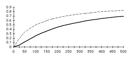
Figure 1 shows how MRPROP varies as additional properties are added to a 100 main subject knowledge base.
Figure 1: Values of MRPROP when there are 100 main subjects. The x axis shows the effect of an increasing number of user properties. The bold plot is that of MRPROP while the dashed plot shows what the metric would look like if it were not squared. The squaring flattens the curve and thus makes the metric more useful.
To summarize, the formula for MDET is as follows:
MDET = MMSSLV / MMSS
where MMSS is the number of main subject statements (statements whose subject is a main subject)
and MMSSLV is the number of main subject statements which have local values
Whereas MRPROP measures the potential number of specialized statements , MDET indicates the amount of use of that potential. The next measure, MSFORM, goes one step further and measures to what degree that use results in the interconnection of concepts.
The formula for MSFORM is as follows:
MSFORM = MMSFS / MMSSLV
where MMSSLV is the number of main subject statements with local values (see MDET)
and MMSFS is the number of main subject formal statements, i.e. those with local values containing value items that are other concepts
The denominator of MSFORM is composed of only those statements that form the numerator of MDET - those statements with locally specified values. It thus should be independent of MDET : i.e. regardless of whether MDET is near zero or near one, MSFORM can still range from zero to one. The one exception is when there are no statement values, in which case MDET is zero and MSFORM is undefined.
The diversity metric, MDIV, measures the degree to which the introduction of properties is evenly spread among main subjects. If all properties are introduced in one place (e.g. at the top concept) then MDIV is close to zero because the knowledge base is judged to be simpler. Likewise, MDIV is close to zero if properties are introduced mostly on leaf concepts (so there is no inheritance). Maximum MDIV complexity of one is achieved when some properties are introduced at the top of the inheritance hierarchy, some in the middle and some at all of the leaves.
The method of calculating MDIV is described in the following paragraphs; figure 2 is used to illustrate the calculations.
To calculate MDIV, the first step is to calculate the standard deviation of the number of properties introduced at each main subject. This is zero if the introduction of properties is evenly distributed, and some higher number otherwise. The next step is to normalize this standard deviation into the range zero to one. The following formula accomplishes this:
MCONCEN = (([[sigma]] PI) / MUPROP) *
where MUPROP is the number of user properties in the knowledge base
and PI is the number of properties introduced at a main subject
and [[sigma]] is the standard deviation operator
A simple way to convert MCONCEN into a diversity metric would be to calculate 1-MCONCEN. However, thus results in measurements being too crowded towards zero. MDIV is actually calculated using the following more subjectively appealing formula:
MDIV = (1 - MCONCEN2)2
Figure 3 plots the relationship between MCONCEN and MDIV.
* The use of metaconcepts, i.e. the concepts that describe concepts themselves
* The use of terms, i.e. symbols that represent things.
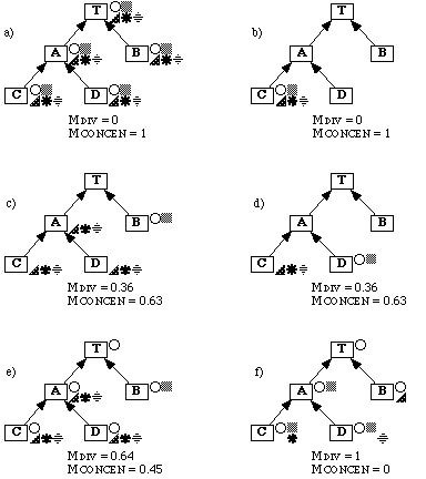
Figure 2: Calculation of MDIV. Each part shows an inheritance hierarchy with five main subjects and five properties (shown as five distinct shapes). Parts a and b show pathological situations where properties are all introduced at a single concept (the top and a leaf respectively) and MDIV is thus zero. Part f shows a well balanced case, where each concept introduces exactly the same number of new properties (one in this case) and MDIV is one. Parts c, d and e show intermediate cases.
Every main subject in principle has a metaconcept, but most are ignored by users. Of interest are those which users have explicitly made the subjects of statements (i.e. those which users have said something about). Similarly, every main subject generally has a term that is used to name it. However, of interest are those cases where extra terms are specified: This indicates that users have paid attention to linguistic issues.
MSOK is zero if the user has neither worked with metaconcepts nor specified synonyms for any concept. The metric gives a measurement of one if every main subject has both multiple terms and metaconcept statements. MSOK is thus calculated as follows:
MSOK = (MFMETA + MFTERM ) / 2
where MFMETA is the fraction of main subjects whose metaconcept has a user-specified statement
and MFTERM is the fraction of main subjects that have more than one term
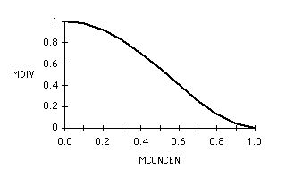
Figure 3: The relationship between MCONCEN and MDIV . MCONCEN, shown in the x axis is a normalized version of the standard deviation of the number of properties introduced at each main subject. This is transformed using a sigmoid function, as plotted in the above graph, in order to obtain a metric that has a good subjective `feel'.
MFLEAF = MLEAF / MTYPES
where MLEAF is the number of leaf types
and MTYPES is the total number of types
For any non-trivial knowledge base, MFLEAF is a function of the branching factor, MBF (2 for a perfect binary tree, 3 for a perfect ternary tree etc.) however the latter is not used as a metric because it is open ended (i.e. not in a zero-to-one range). The formula relating branching factor to MFLEAF is as follows:
Lim MFLEAF = (MBF - 1) / MBF
MTYPES->[[infinity]]
where MTYPES is the total number of types
Figure 4 shows several simple inheritance hierarchies along with their measures of MFLEAF. MFLEAF approaches 0.5 when the inheritance hierarchy is a binary tree (figure 4, parts c and f). It approaches zero in the ridiculous case of a unary `tree' with just a single superconcept-subconcept chain (part b) and it approaches one if every concept is an immediate subconcept of the top concept (part a).
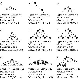
Figure 4: Complexities of various inheritance hierarchies. Parts a through i show increasing complexity using the MISA metric. Parts a and b show simplistic cases (MISA would be small regardless of the size of the knowledge base). Parts c and d show the same structure, with variation only in multiple inheritance. Pairs (e,f) and (g,h) also show similar structures with variation in multiple inheritance, however MISA can be seen to be somewhat independent of the adding of extra parents (such an action may either increase or decrease MISA ).
On its own, MFLEAF has the undesirable property that for a very shallow hierarchy (e.g. just two or three levels) with a high branching factor it gives a measurement that is unreasonably high, from a subjective standpoint (part a of figure 4 illustrates this)
To correct this problem with MFLEAF , an additional factor is used in the calculation of MISA: the average number of direct and indirect superconcepts per non-root main subject , MALLSUP. (The root concept at the top if the inheritance hierarchy is not counted since it cannot have parents). This second factor is related to hierarchy depth but depends to some extent on the amount of multiple inheritance.
MISA is thus calculated using the following formula:
MISA = MFLEAF - (MFLEAF / MALLSUP)
MISA approaches zero in either of the following cases: 1) when there is just a single layer of concepts below the top concept (no matter how many concepts); or 2) when the branching factor is one. MISA approaches the value of MFLEAF (e.g. 0.5 for a binary tree) as the hierarchy becomes deeper (as the average number of direct or indirect parents per main subject increases).
MMI measures the ratio of extra parents to main subjects, thus if all main subjects had two parents (impossible in fact because the concepts directly below the top concept cannot have more than one parent) then the metric would be one; it could also be one if a substantial number of concepts have more than two parents. Although the metric, as described, could theoretically give a value above one, it is assumed that this could not be the case in any reasonable knowledge base. Thus a ceiling of one is imposed that the metric cannot exceed, even if there are an excessive number of parents.
The generic procedure for designing a compound metric is as follows:
1) Choose the metrics that are to be combined by looking for those with certain desired characteristics.
2) Normalize the metrics so that they are not arbitrarily biased.
3) Weight the metrics based on decisions about which are most important, and how much their values should contribute to the resulting metric
4) Design a formula that combines the metrics.
Although both step 2 and step 3 involve finding coefficients that modify the original values of the metrics, they are logically separate steps. After step 2, accidental bias is removed. Such bias may be caused by the fact that the metrics might have quite different expected values or ranges. In step 3, deliberate weighting is added. For this initial research, step 3 is ignored since it would require a very large amount of data to justify an unequal weighting. The most important step in this research is step 4.
The metrics chosen to compose MACPLT are:
* MRPROP, indicating the extent to which properties have been added
* MDET, indicating the proportion of potential statements with actual values, and
* MSFORM indicating the extent to which the knowledge base has been formalized.
The possibility of adding MSOK was considered, but it was decided not to do this because the amount of second order knowledge might be heavily dependent on the domain, whereas the extent to which statements are filled in and formalized appears much more likely to measure the state of completeness, independent of domain.
To remove accidental bias from the metrics, actual knowledge bases were studied to see how the component metrics range in practice (see section 6). None ever approached a value of one, and the maximums for well-worked out knowledge bases were all about 0.7. It seems reasonable that none of these metrics would ever reach one for the following reasons:
* MRPROP can only asymptotically approach 1 as ever larger numbers of properties are added. A measurement as high as 0.7 already indicates that there are over five times as many properties as main subjects. Experience has shown that it is unlikely for a knowledge base to have a much higher proportion of properties than this.
* If MDET were to approach 1, it would mean that hardly any statements are inherited; all would be locally specified (i.e. they all override inherited values). This seems unlikely to happen in most knowledge bases.
* If MSFORM were to approach 1, the user has been able to formalize all statements. This seems unlikely in a normal knowledge base.
It was thus decided that prior to combining the metrics to create MACPLT , all of them should be normalized so that when a measure using the normalized metric has a value of about 1, it is considered to indicate that the particular aspect of the knowledge base is reasonably complete. It is purely coincidental that the 0.7 is used for all three: All three component metrics all had measured ranges of 0-0.7.
The coefficient used to normalize the metrics is the reciprocal of 0.7, i.e. 1.4. As a result of this, MACPLT can give measurements greater than one - that would merely indicate that more detail has been provided than in a normal complete knowledge base.
The following points explain how it was decided to combine the metrics:
* MRPROP must dominate the calculation for the following reason: If there are few properties, then high measurements of detail and formality mean little (because there can only exist a few statements with potential for having detail and formality). Thus MRPROP should be a multiplicative value for the whole metric formula - if MRPROP is zero then MACPLT should be zero.
* For similar reasons, MDET must dominate MSFORM. If there are few statements, then a high measurement of formality means little because there are only a few statements to be formal.
The basic formula for combining the three metrics is therefore:
MACPLT = C * MRPROP * ( W + C * MDET * ( X + Y * C * MSFORM))
Where C is the constant 1.4 used to unbias the metrics; i.e. to convert their 0 to 0.7 range to a range of 0 to 1. If this factor were missing , the resulting metric could only yield measurements that would approach 70%.
And where W, X and Y are coefficients used to weight the metrics. As discussed earlier it was decided to weight the metrics equally. These three coefficients should all be 0.33 then. That would mean that if all three input metrics approached one, the result would be 0.33 * 3 = 1.
Simplifying the above, where Z is used in place of W, X and Y, gives:
MACPLT = MRPROP * (C * Z + MDET * (C2 * Z + C3 * Z * MSFORM))
After application of the constants, the derived formula for MACPLT is thus as follows:
MACPLT = MRPROP * (0.47 + MDET * (0.65 + 0.91 * MSFORM))
An interesting derivative use of MACPLT would be to apply it to different subhierarchies of a knowledge base in order to determine which areas need work, or alternatively, which areas contain more useful knowledge.
To calculate adjusted function points, the first step is to measure fourteen complexity adjustment factors using simple scales and then to sum the measurements (without weighting). The sum can be called the `compound adjustment factor'. In the second step, a formula involving the compound adjustment factor results in the multiplication of the unadjusted function points by a factor ranging from 0.65 to 1.35. In the following paragraphs, a similar two-step approach is applied to knowledge base metrics.
Step 1: Scaling and summing. The four metrics not included in MMACPLT have theoretical ranges of zero-to-one. However, upon examining data from user studies, it was determined that measurements of three of the four metrics rarely approach the top of that range (MSOK is the exception).
Thus it was decided to apply multiplicative scaling factors to MSOK, MISA and MMI in order to unbias them (so that each metric contributes fairly to the result). The scaling factors (2.5, 1.6 and 1.2 respectively) were determined by examining the means and ranges of the test data. These scaling factors are the least objective aspect of the calculation of MPCPLX - extensive data analysis would be needed to fine tune them; however since this research is intended to propose a method for developing metrics rather than a definitive formula, these figures are considered adequate. The resulting compound adjustment factor has a range of zero to four (see formula below).
Step 2: Creating the adjusted metric: It was decided to adjust MMACPLT so that the resulting metric is MMACPLT multiplied by between 0.25 and 1.85. This is a wider range than that used for function points, but it was decided the four adjustment factors should have a larger influence than those used for function points. Again, more extensive data analysis would be needed to arrive at a more objective range.
The derived formula for MPCPLX is thus as follows:
MPCPLX = MMACPLT * (0.25 + 0.4 *
(MDIV + 2.5 * MSOK + 1.6 * MISA + 1.2 * MMI))
where the second line is the compound adjustment factor
* All concepts: MALLC: This gives an idea of the amount of memory and disk space used by the knowledge base. It also gives an idea of the number of discrete facts in the knowledge base.
* Main subjects: MMSUBJ: This indicates to the user the number of things being talked about in the knowledge base, and hence is a natural measure of size that is independent of complexity. If the user follows a methodology of sketching out the inheritance hierarchy before filling in details, this metric can help him or her estimate the eventual size of the knowledge base and hence the amount of work that might be required to create it.
* Relative Properties: MRPROP: This indicates to the user whether a knowledge base has a reasonable number of properties, relative to the number of main subjects. A low measurement might indicate that more properties should be added.
* Detail: MDET: This indicates whether a knowledge base (or portion thereof) has a reasonable number of statements. A low measurement might suggest that additional statements should be added.
* Statement Formality: MSFORM: This indicates whether a knowledge base has a reasonable number of formal links. A low measurement indicates that the user would be unlikely to be able to generate sophisticated graphs of relations.
* Diversity: MDIV: This indicates the degree to which knowledge is focused at the top or bottom of the inheritance hierarchy. A low value might indicate that inheritance is not being properly used and that many concepts are merely placeholders.
* Second Order Knowledge: MSOK: This indicates the extent to which knowledge is included about concepts themselves as opposed to the things represented by concepts. A low measurement indicates that there is probably significant knowledge missing.
* Isa Complexity: MISA: This metric indicates the degree to which the inheritance hierarchy has a non-trivial pattern of branching. A low measurement indicates that many concepts do not have siblings and thus relatively few distinctions are being made.
* Multiple inheritance: MMI: This indicates the extent of the complexity added due to multiple inheritance. A low measurement indicates that little multiple inheritance is being used.
* Apparent completeness: MACPLT: By combining those metrics that should logically increase as a knowledge base approaches completion, this metric gives the user an idea of how close to completion the knowledge base might be.
* Pure complexity: MPCPLX: By combining all the complexity metrics this gives the user an overall value of the `difficulty' of the knowledge base, independent of size.
* Overall complexity: MOCPLX: In combining pure complexity with size, this metric is intended to give the user an idea of the information content in a knowledge base.
The methods of calculating MALLC and MMSUBJ are the simplest, being mere counts. MDET, MSFORM and MMI have a slightly lower level of understandability since they are simple ratios of reasonably understandable counts. MRPROP is lower again in understandability since it is squared in order to give it better responsiveness to the underlying phenomenon. The other metrics all have relatively complex formulas.
One test of correspondence for metrics with a zero-one range is as follows: The metric should yield a value of 0.5 when the subjective phenomenon is at about the half-way point, i.e. the subjectively `normal' point. Another test is to ensure that the endpoints correspond with what one would intuitively expect. Table 1 gives interpretations for the endpoints and centre points of the closed-ended metrics and shows that they behave well in these respects. The only possible exception is MRPROP whose middle point indicates that there are 2.5 properties per concept - however this occurs in order to ensure that equal deltas of the metric correspond more closely with equal changes in the subjective phenomenon.
Metric        Meaning approaching   Meaning near 0.5      Meaning approaching
              0                                           1
  MRPROP      No properties         2.5 properties per    Very many
                                    concept               properties per
                                                          concept
  MDET        No values specified   Values specified on   Value specified
                                    half of statements    wherever possible
  MSFORM      No formal values      Half of values are    All values are
                                    formal                formal
  MDIV        Properties            Properties            Properties
              introduced on one     introduced on half    introduced evenly
              concept               of all concepts       on all concepts
  MSOK        No second order       Metaconcept detail    Both metaconcept
              knowledge             and extra terms on    detail and extra
                                    about half of         terms on every
                                    concepts              concept
  MISA        Each concept has      Binary tree           Very bushy tree -
              about one parent -                          very complex
              very simple
  MMI         No multiple           Half of concepts      Very high degree of
              inheritance           have an extra parent  multiple inheritance
Table
1: Interpreting metrics - meanings of various values. Rows show metrics defined
that are closed-ended. Columns indicate the interpretation of measurements at
the extremes of that range and in the middle.
The following are some other general observations about the metrics:
* The most useful metrics appear to be MOCPLX, MDET and MSFORM. User studies (section 6) showed that the overall complexity metric correlates reasonably well with time-to-complete, whereas MDET and MSFORM give clear indications of where work needs to be done in a knowledge base.
* The metrics that have the best combination of understandability and usefulness are MMSUBJ and MDET.
* Most metrics correspond well with subjective phenomena.
* All the metrics with a zero-to-one range have good meanings for the ends of the ranges
                     Suitable
Task                 Metrics         Observations
A to D. Assessing the present state of a knowledge base
 Completeness        MACPLT          The compound metric of apparent
                                     completeness.
 Complexity          MPCPLX, MDET,   Pure complexity, and two of its most
                     MSFORM          important components: detail and
                                     statement formality
 Information         MOCPLX          The overall complexity of the knowledge
content                              base
 Balance             MDIV            The diversity of distribution of
                                     properties; other balance metrics could
                                     be created.
E. Predicting        MMSUBJ          The number of main subjects can typically
                                     be determined earlier than other metrics
F to I. Comparing    all
Table
2: Measuring tasks and how well they can be performed. At the left are the
measuring tasks listed in section 5.3. The middle column lists some of the
metrics that may be useful in the performance of the task.
For this work, the following procedure was used:
1. 12 people who were interested in building knowledge bases in CODE4 were selected as participants. These included 11 graduate students and one professor.
2. The participants were trained to use the system. They also had access to a 100 page user manual .
3. They created 25 knowledge bases, covering such topics as:
* Computer languages and operating systems.
* Other technical topics (such as optical storage, electrical devices, geology and matrices)
* General purpose knowledge (people, vehicles etc.)
The total amount of work involved in creating the knowledge bases was about 2000 hours, i.e. an average of 80 hours per knowledge base.
4. The participants were asked to complete a questionnaire about their experiences. This questionnaire contained 55 main questions and, among other things, asked for the participants' subjective impressions of the complexity and completeness of their knowledge bases.
5. The resulting knowledge bases were measured using the simple complexity metrics developed in this paper. The same knowledge bases were also used to calibrate the compound complexity metrics.
Metric                  Theoretical     Mean     Minimum      Maximum     Standard
                              Range                                      Deviation
Raw size metrics
  All concepts: MALLC        (40-[[      842         224         2825          612
                             infini
                             ty]])
  Main subjects: MMSUBJ      (0-[[i       91          21          278           61
                             nfinit
                             y]])
Independent complexity
metrics
  Relative Properties:       (0-1)      0.33        0.05         0.70         0.17
MRPROP
  Detail: MDET               (0-1)      0.18        0.03         0.69         0.14
  Statement Formality:       (0-1)      0.16        0.00         0.67         0.19
MSFORM
  Diversity: MDIV            (0-1)      0.71        0.00         0.99         0.27
  Second Order Knowledge:    (0-1)      0.06        0.00         0.41         0.11
MSOK
  Isa Complexity: MISA       (0-1)      0.40        0.19         0.59         0.11
  Multiple inheritance: MMI  (0-1)      0.19        0.00         0.87         0.23
Compound complexity metrics
  Apparent completeness:     (0-2)      0.20        0.03         0.39         0.11
MACPLT
  Pure complexity: MPCPLX    (0-5.6     0.19        0.02         0.38         0.10
                             )
  Overall complexity:        (0-[[i       16           2           56           14
MOCPLX                       nfinit
                             y]])
Table
3: Statistics about knowledge bases created by the participants. Each row
corresponds to one of the metrics discussed in section 4.The following are some general observations about table 3:
* The knowledge bases differ substantially in size. When measured using MALLC and MMSUBJ the ratio of largest to smallest is about 13:1. When measured using MOCPLX, however, a more realistic ratio appears, i.e. 28:1.
* The knowledge bases vary widely according to all of the independent complexity metrics, in particular according to MDIV and MMI. Of these, MDIV is probably the most interesting since it seems to be more of an indicator of the individual style of the knowledge base developer than the other metrics.
As table 4 indicates, for the most part success has been achieved. The biggest exception is the reasonably strong negative correlation between the isa complexity and the amount of multiple inheritance. This can be accounted for theoretically because if there are more parent concepts to be multiply inherited (including by leaves), then the proportion of leaf types should decrease.
                            Multipl      Isa   Second  Diversi  Statement  Detai
                                  e  Complex    Order       ty  Formality      l
                             Inher.        .
                                MMI     MISA     MSOK     MDIV     MSFORM   MDET
      Relative Properties:     0.15    -0.23     0.11    -0.13      -0.17   0.17
                    MRPROP
              Detail: MDET     0.12    -0.28    -0.21    -0.06      -0.16
      Statement Formality:    -0.19     0.04    -0.02     0.34
                    MSFORM
           Diversity: MDIV    -0.18     0.07    -0.08
   Second Order Knowledge:    -0.21     0.14
                      MSOK
Isa complexity: MISA          -0.58
Table
4: Coefficients of linear correlation among the seven complexity metrics. The
data used in calculating these coefficients was obtained from the knowledge
bases prepared by the participants.
This paper has discussed several metrics that can be applied to frame-based knowledge representations. The metrics can be divided into three classes: 1) raw measures of size; 2) measures of various attributes of complexity, and 3) compound measures intended to help users assess their productivity.
With the help of metrics, users can better do such things as the following:
1. Estimate completeness of a knowledge base, or a component thereof. Using a metric like MACPLT, a user can decide how much work might need to be done and where.
2. Judge the overall volume of knowledge in a knowledge base, using MOCPLX.
3. Obtain a rough idea of how difficult a knowledge base might be to navigate or modify; MPCPLX can help with this.
4. Compare subjectively `complete' knowledge bases to see how domains differ, in order to help in the estimation of future knowledge base development tasks.
The main scientific contribution of this paper has been to point out several kinds of things that one might wish to measure in a knowledge base. It is hoped that the work will stimulate people to actually measure the products of knowledge engineering and to perform further research into metrics.
2. D. Skuce and T. C. Lethbridge, "CODE4: A Unified System for Managing Conceptual Knowledge", Int. J. Human-Computer Studies 42 (1995), 413-451.
3. T.C. Lethbridge, Practical Techniques for Organizing and Measuring Knowledge, Ph.D. thesis, Department of Computer Science, University of Ottawa, 1994.
4. I. Meyer, K. Eck and D. Skuce, "Systematic Concept Analysis Within a Knowledge-Based Approach to Terminology", in Handbook of Terminology Management, Eds. S.E. Wright and G. Budin, John Benjamin, 1994.
5. J. Bradshaw, P. Holm, O. Kiperztok and T. Nguyen. "eQuality: A Knowledge Acquisition Tool for Process Management", Proc. FLAIRS 92, Fort Lauderdale.
6. M. Longeart, G. Boss and D. Skuce, "Frame-based Representation of Philosophical Systems Using a Knowledge Engineering Tool", Computers and the Humanities 27 (1993), 27-41.
7. B. Porter, J. Lester, K. Murray, K. Pittman, A. Souther, L. Acker and T. Jones, AI Research in the Context of a Multifunctional Knowledge Base: The Botany Knowledge Base Project, Technical Report, The University of Texas at Austin.
9. D. Lenat and R. Guha, Building Large Knowledge Based Systems, Addison Wesley , 1990.
9. R. Brachman, D. McGuiness, P. Patel-Schneider, L. Resnick and A. Borgida, "Living with CLASSIC: When and How to Use a KL-ONE Like Language", in Principles of Semantic Networks, Ed. J. Sowa, Morgan Kaufmann, 1991, pp. 401-456.
10. M. Shepperd and D. Ince, Derivation and Validation of Software Metrics, Oxford, 1993.
11. T.J. McCabe, "A Complexity Measure", IEEE Trans. Software Eng. 2 (1976), 308-320.
12. S.M. Henry and D. Kafura, "Software Structure Metrics Based on Information Flow," IEEE Trans. Software Eng., 7 (1981), 510-518.
13. G. C. Low and D. R. Jeffrey, "Function Points in the Estimation and Evaluation of the Software Process", IEEE Trans. Software Eng. 16 (1990), 64-71.
14. V.R. Basili and H.D. Rombach, "The TAME Project: Towards Improvement-Oriented Software Environments," IEEE Trans. Software Eng. 14 (1988), 758-773.
15. L. Acker, Access Methods for Large, Multifunctional Knowledge Bases, TR AI92-183, Ph.D. Thesis, Department of Computer Science, University of Texas at Austin, 1992.
16. B.W. Boehm, Software Engineering Economics, Prentice-Hall, 1981.